2 Network exploration

This chapter demonstrates how to explore the reference networks of corticogenesis, neurogenesis and gliogenesis. It provides the code chunks to reproduce the results of the paper figures and examples on how to use the resource.

2.1 Quickstart

These are the main functions to load, visualize, and inspect the complete corticogenesis resource.

#STEP 1: load package
library(neuRoDev)

#STEP 2: load data 
corticogenesis_sce <- corticogenesis.sce(directory = '~/Downloads')
neurogenesis_sce <- neurogenesis.sce(directory = '~/Downloads')
gliogenesis_sce <- gliogenesis.sce(directory = '~/Downloads')

#STEP 3: plot network
plotNetwork(net = corticogenesis_sce)
plotNetwork(net = neurogenesis_sce)
plotNetwork(net = gliogenesis_sce)

#STEP 4: plot network stages
plotNetwork(net = corticogenesis_sce, 
            color_attr = 'Stages')
plotNetwork(net = neurogenesis_sce, 
            color_attr = 'Stages')
plotNetwork(net = gliogenesis_sce, 
            color_attr = 'Stages')

#STEP 5: plot eTrace
plot_eTrace(corticogenesis_sce, 
            genes = 'SST')
plot_eTrace(neurogenesis_sce, 
            genes = 'CUX2')
plot_eTrace(gliogenesis_sce, 
            genes = 'SPARCL1')

Below we present a more detailed overview of the different tools and functions.

2.2 Loading necessary libraries and data

2.2.1 Loading the right libraries

# functions package
library(neuRoDev)
# extra packages
library(SingleCellExperiment)
library(gtools)

2.2.2 Loading the networks necessary objects

The data used in this tutorial can be downloaded here. The functions corticogenesis.sce, neurogenesis.sce, and gliogenesis.sce can be used to directly download the data and/or load the data. By default, the functions download the data in the neuRoDev cache folder, but a custom directory can be defined by changing the directory variable. The function checks whether the file is already present and, if not, downloads it.

corticogenesis_sce <- corticogenesis.sce(directory = '~/Downloads')
neurogenesis_sce <- neurogenesis.sce(directory = '~/Downloads')
gliogenesis_sce <- gliogenesis.sce(directory = '~/Downloads')

If someone wants to start from the count matrices, we have stored them as a unique matrix and the associated metadata that can be downloaded from here (SingleCellCompendium folder).

The reference datasets comprise:

signatures: this contains the sample-wise signatures (relative expression levels) of each cluster.
logcounts: this contains the normalized pseudobulk expression of each cluster.
colData: here are saved all the information about the networks, including the name of each cluster, the study, its age in days and stages, its subclass/subtype, starting class and subclass annotation (RefClass and RefSubClass), x and y UMAP coordinates, etc.
correlations: it contains all the correlation values between cluster signatures and cell type reference signatures. Saved in metadata.
network: it comprises the edges, the distances, the adjacency matrix, and indexes. Saved in metadata.
subclass_psb: this contains as an additional SingleCellExperiment object the subclasses’ pseudobulk logcounts and preferential expression. Saved in metadata.
stage_psb: this contains as an additional SingleCellExperiment object the stages’ pseudobulk logcounts and preferential expression. Saved in metadata.

With this we can start the analysis and the exploration of the reference networks.

2.3 Network visualizations

2.3.1 SubClass (or SubClass) labels and colors

Here we show how it is possible to visualize in the network the different cell types and the age of each cluster.

The network-specific dataframes retain information such as the cluster name, the stage, the age in days, the original label, our annotations etc. Here we show just part of this table:

#> Warning: package 'htmltools' was built under R version
#> 4.4.3

First, we can visualize the UMAP plot of the networks, which is build upon the correlations to the reference signatures. To color the clusters we can provide the labels and their associated color, thus making possible to visualize any kind of cluster-wise label. By default it uses SubClasses.

To plot the network we can use plotNetwork, which requires:

net = the SingleCellExperiment object.
color_attr = the column used to define the annotations used to color the plot. Defaults to “SubClass”.
label_attr = the column used to define the annotations used to label the plot. Defaults to “SubClass”.
col_vector = the color palette to use to color the plot. Defaults to SubClass_color, an internal palette.

The output will show the 2D-UMAP representation of the networks, in which each dot is a single cluster.

plotNetwork(net = corticogenesis_sce)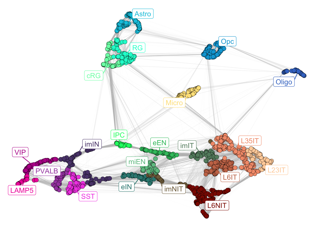

Figure 2.1: Corticogenesis subclasses.

plotNetwork(net = neurogenesis_sce)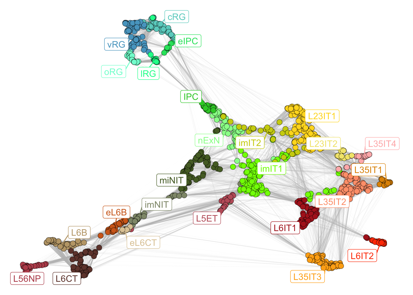

Figure 2.2: Neurogenesis subclasses.

plotNetwork(net = gliogenesis_sce)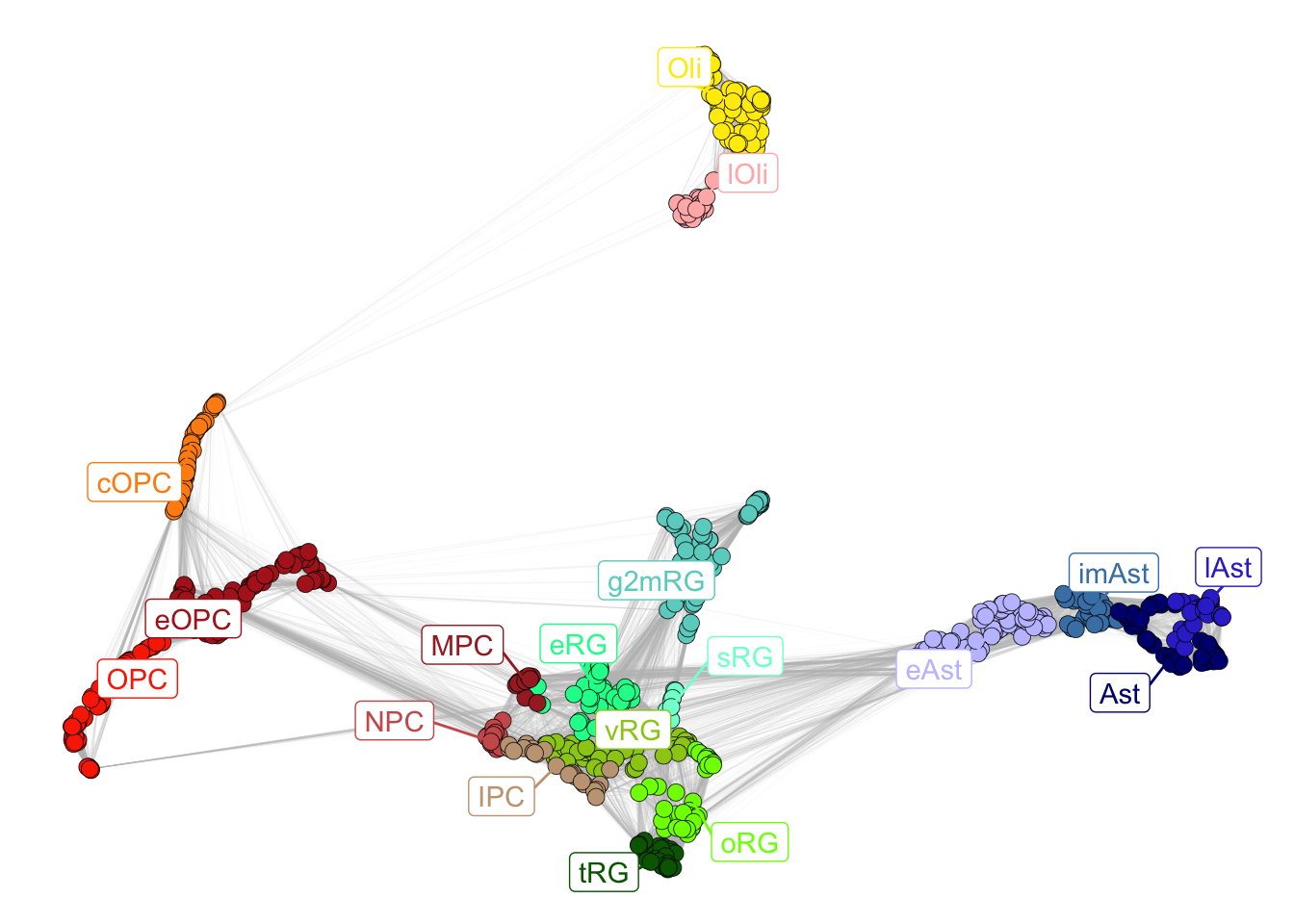

Figure 2.3: Gliogenesis subclasses.

To show the stage of maturation of each cluster, we can plot the network and just modify the color_attr to match the stages. By default the label shown is the subclass colored by the most representative stage. To show the stage label, it is possible to pass “Stages” in the label_attr parameter.

Interestingly, the clusters capture an age gradient that from the center of the network spreads towards the edges. This trend is detectable also within a single subclass, showing that patterns of expression are continuous in time.

plotNetwork(net = corticogenesis_sce, 
            color_attr = 'Stages')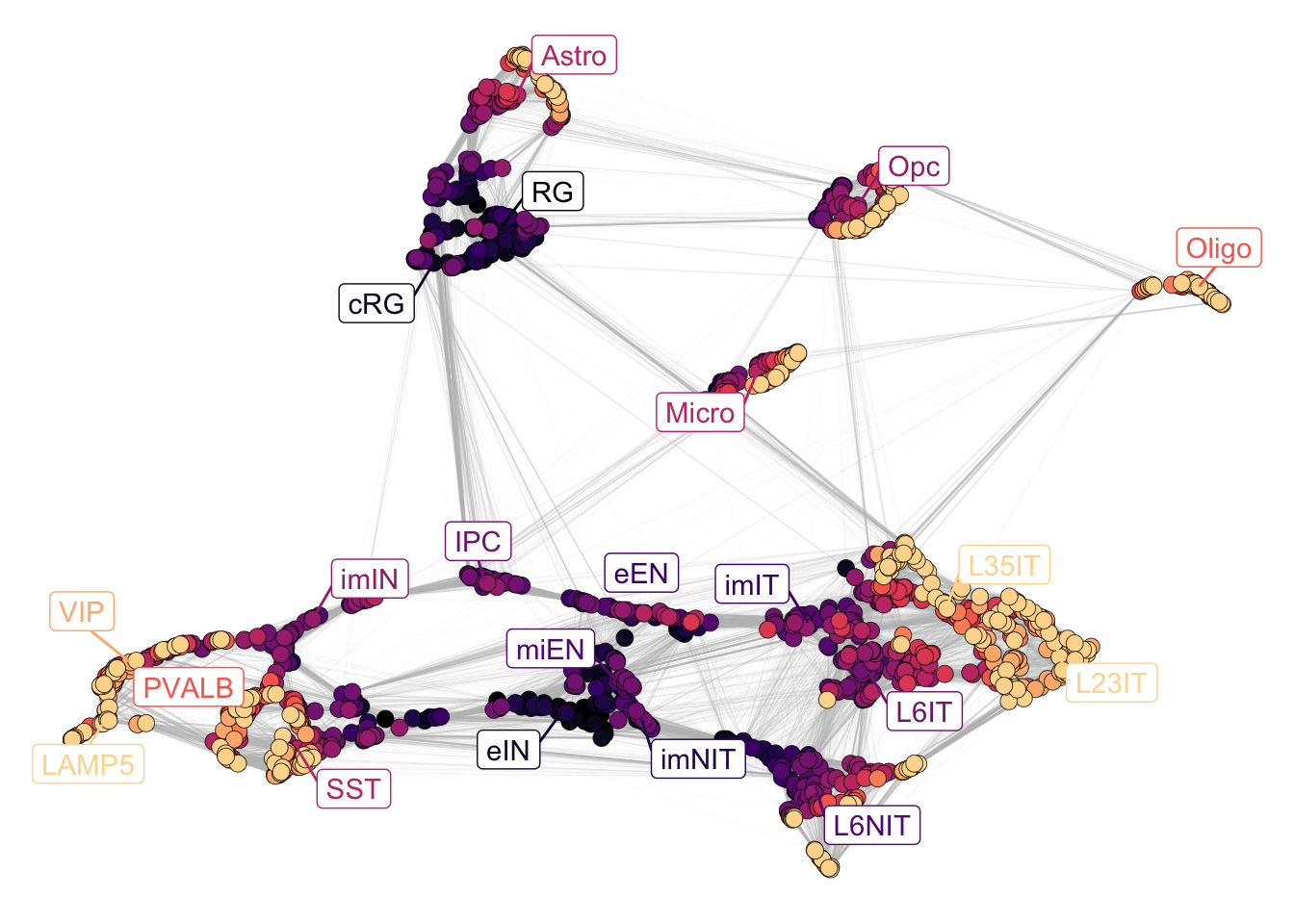

Figure 2.4: Corticogenesis stages.

plotNetwork(net = neurogenesis_sce, 
            color_attr = 'Stages')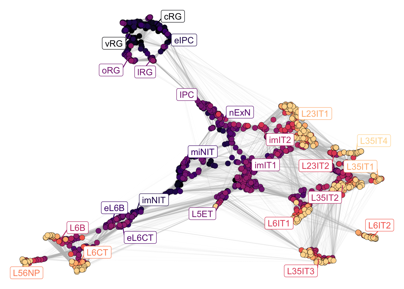

Figure 2.5: Neurogenesis stages.

plotNetwork(net = gliogenesis_sce, 
            color_attr = 'Stages')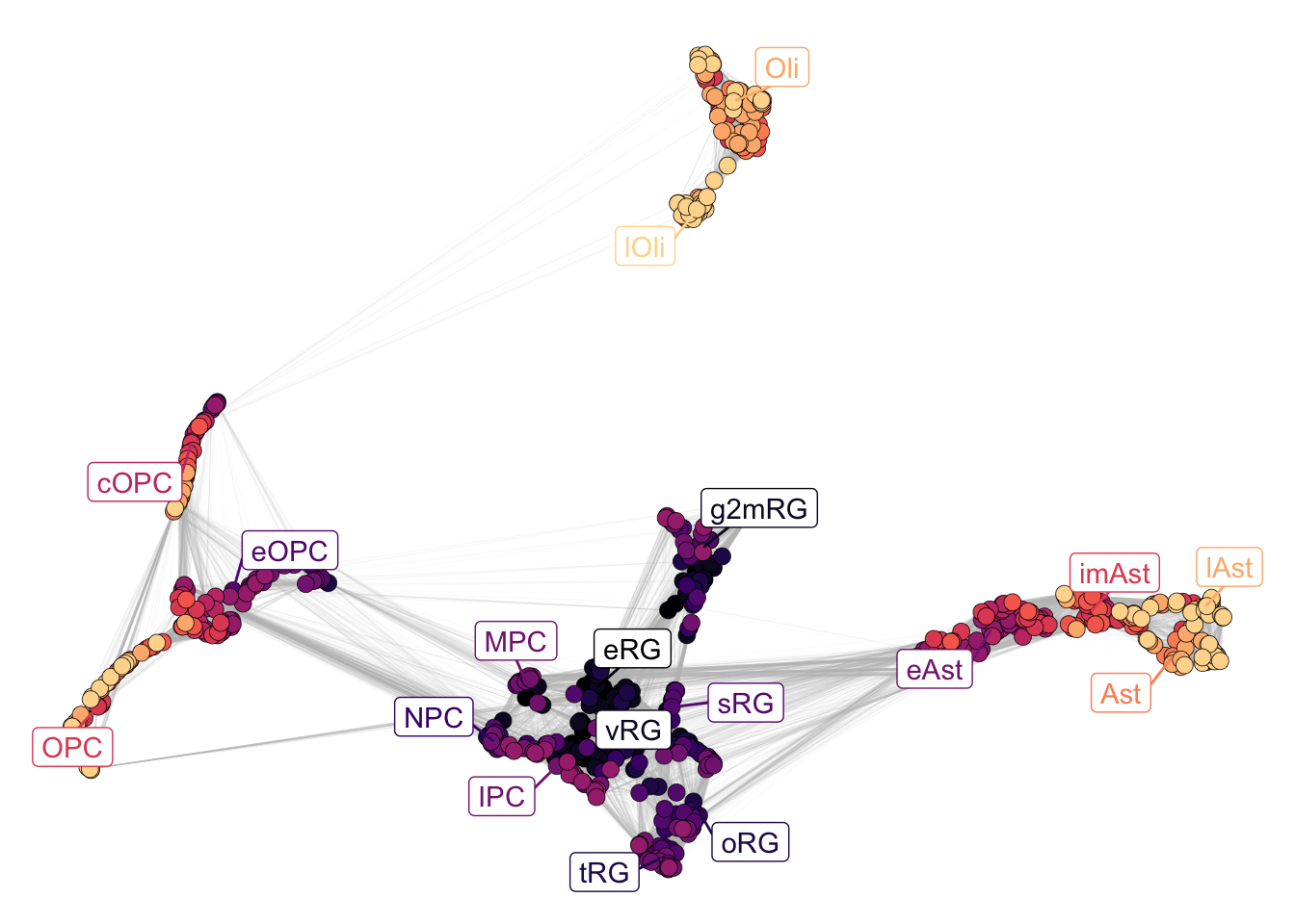

Figure 2.6: Gliogenesis stages.

2.4 Visualize the expression of genes or gene sets

For each cluster we computed its pseudobulk profile. With this, we can explore gene expression in the network with plotNetworkScore.

This function shows the absolute expression level by default, but it can plot any numerical vector across the network, including expression enrichment. The absolute value can be displayed as either raw or smoothed (it considers the network structure and leads to more homogeneous values between clusters in the same neighborhood). The inputs are:

net = the SingleCellExperiment object.
genes= a specific gene or set of genes from which to derive the score to plot. If more genes are given, the output will be an averaged score of those genes. It defaults to NULL, as the user can directly provide a score per cluster (see score). If no genes are given and a score matrix is selected, all genes in the score matrix will be considered.
score= it can be a vector, with one value per cluster, or a matrix. If a matrix is given together with genes (see genes), only the values of the selected genes that are present in the matrix will be shown. It defaults to the log-normalized expression values contained in net under logcounts.
expression_enrichment = whether or not to compute expression enrichment of the genes (only if score if NULL). Defaults to FALSE. For a more detailed description of expression_enrichment, see Chapter Analysis tools.
label_attr = the column used to define the annotations used to label the plot. Defaults to “SubClass”.
smooth = whether or not to smooth the values based on the network structure. Defaults to TRUE
Additional plotting parameters (see ?plotNetworkScore).

The output will show the 2D-UMAP representation of the networks, in which each dot is a single cluster, colored based on the given score.

# no smoothing - one gene - no labels
plotNetworkScore(net = corticogenesis_sce,
                 genes = 'VIP',
                 smooth = FALSE,
                 main = "raw expression")

# smoothing considering 20 neighbors - one gene - no labels
plotNetworkScore(net = corticogenesis_sce,
                 genes = 'VIP',
                 smooth = TRUE, 
                 n_nearest = 20,
                 main = "smoothed expression")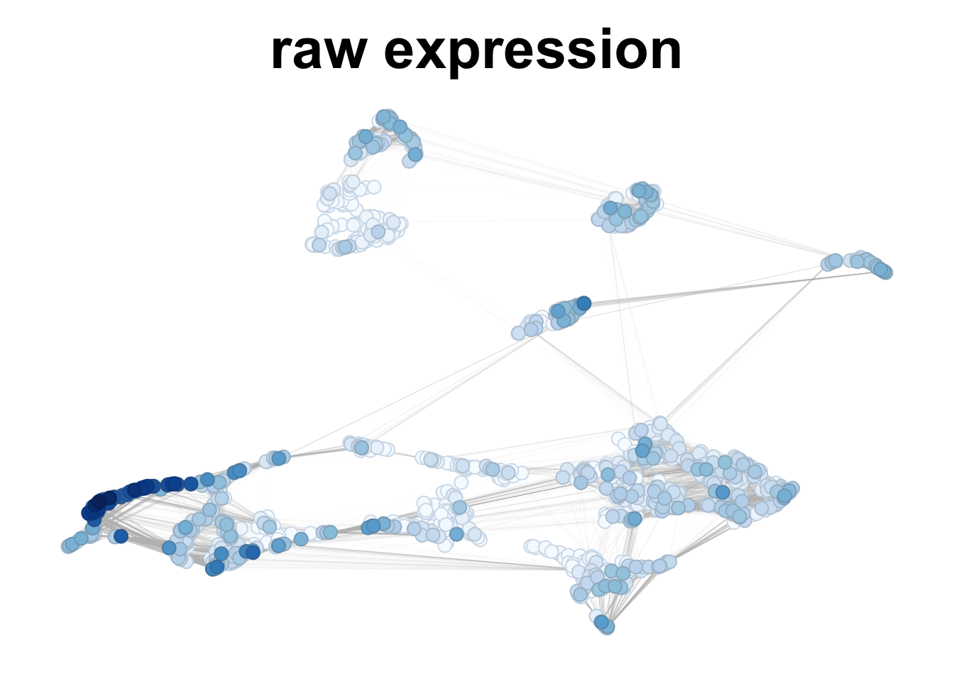

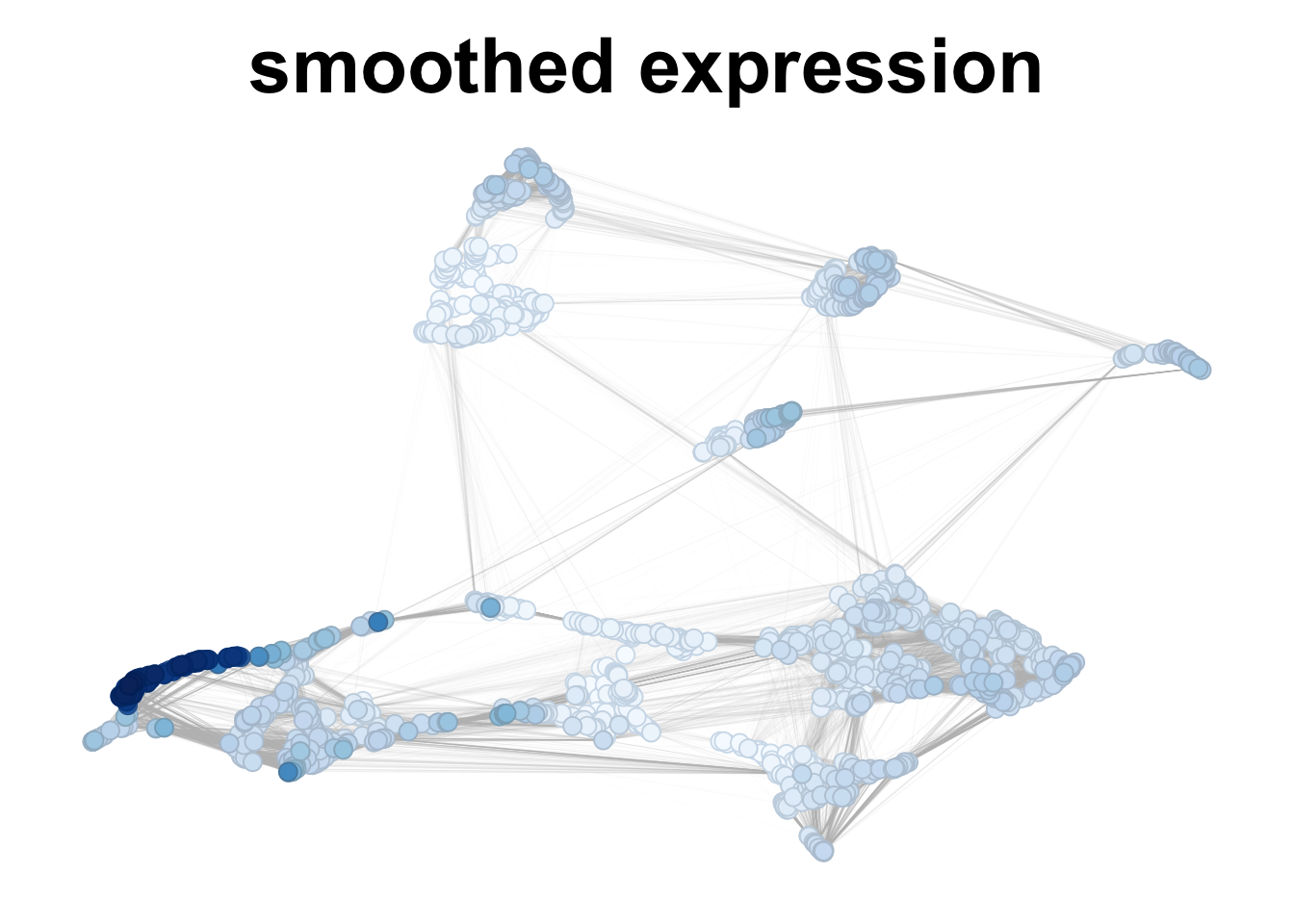
Figure 2.7: VIP gene expression in corticogenesis, without and with smoothing.

plotNetworkScore(net = neurogenesis_sce,
                 genes = 'NEUROD6',
                 smooth = TRUE, 
                 n_nearest = 20)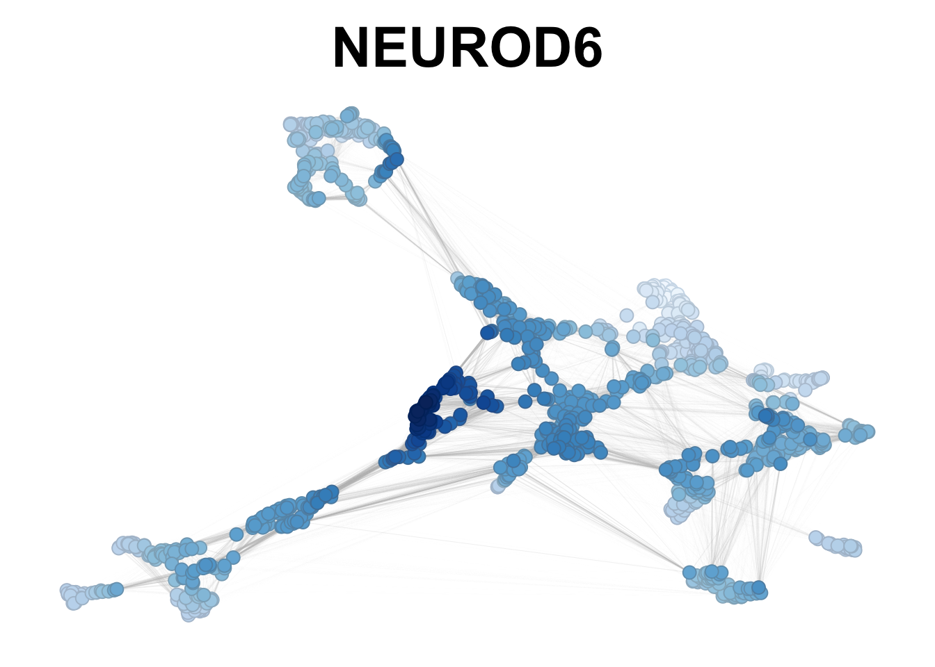

Figure 2.8: NEUROD6 smoothed expression in neurogenesis.

plotNetworkScore(net = gliogenesis_sce,
                 genes = 'OLIG1',
                 smooth = TRUE, 
                 n_nearest = 20)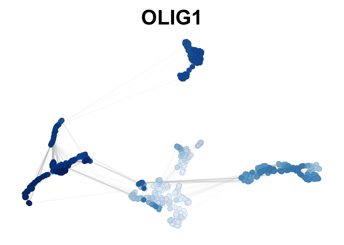

Figure 2.9: OLIG1 smoothed expression in gliogenesis.

This is an example of preferential expression:

plotNetworkScore(net = gliogenesis_sce,
                 genes = 'GFAP',
                 expression_enrichment = TRUE,
                 smooth = TRUE, 
                 n_nearest = 20)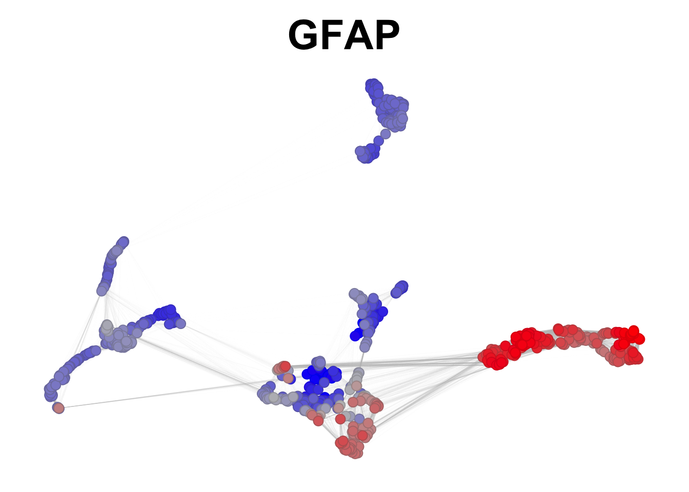

Figure 2.10: GFAP preferential expression in gliogenesis.

We can also look at the average expression of specific group of genes of interest. Here we show some manually selected cell cycle genes in the network.

#manually selected cell cycle genes
cell_cycle_genes <- c(
  "CCND1", "CCND2", "CCND3", "CCNE1", "CCNE2", "CCNA2", "CCNB1", "CCNB2",
  "CDK1", "CDK2", "CDK4", "CDK6",
  "CDKN1A", "CDKN1B", "CDKN2A", "CDKN2B"
)

plotNetworkScore(net = corticogenesis_sce,
                 genes = cell_cycle_genes,
                 smooth = TRUE, 
                 n_nearest = 20,
                 main = "Cell cycle")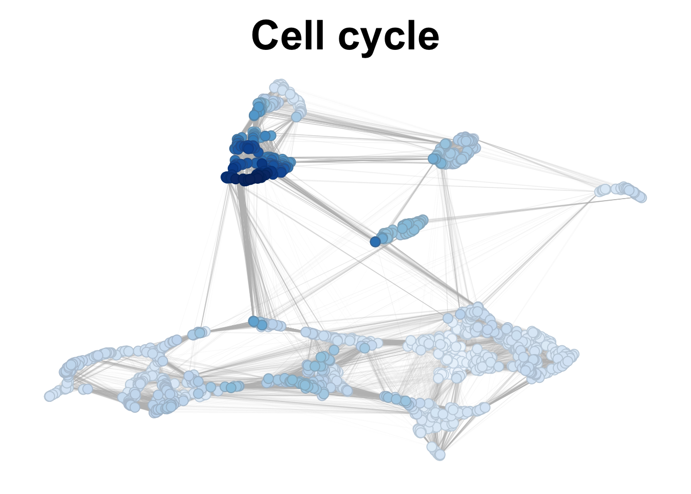

Figure 2.11: Cell cycle genes expression in corticogenesis.

2.5 SubClass composition across ages

Cortical development is a highly dynamic process in which cell types appear at distinct stages as progenitor populations shift their fate over time. To explore how this happens, we can look at the cell type composition in time.

2.5.1 Proportions across ages

To assess how the subclasses change in time, we can take a look at how their proportions evolve, leveraging our knowledge of both cell type and developmental time.

Show the code (ordering age)

unique_ages <- mixedsort(unique(corticogenesis_sce$Age))
ordered_ages <- c(unique_ages[grep('w', unique_ages)], 
                  unique_ages[grep('d', unique_ages)], 
                  unique_ages[grep('m', unique_ages)], 
                  unique_ages[grep('yr', unique_ages)])

stages.indexes <- unlist(lapply(mixedsort(unique(as.vector(corticogenesis_sce$Stages))), function(i) {
  strsplit(i, "-")[[1]][1]
  }))

Show the code (lineages proportion in time)

corticogenesis_subclass_proportion <- table(corticogenesis_sce$SubClass, corticogenesis_sce$Age)

corticogenesis_subclass_proportion <- t(t(corticogenesis_subclass_proportion)/colSums(corticogenesis_subclass_proportion))


neurogenesis_subclass_proportion <- table(neurogenesis_sce$SubClass, neurogenesis_sce$Age)

neurogenesis_subclass_proportion <- t(t(neurogenesis_subclass_proportion)/colSums(neurogenesis_subclass_proportion))


gliogenesis_subclass_proportion <- table(gliogenesis_sce$SubClass, gliogenesis_sce$Age)

gliogenesis_subclass_proportion <- t(t(gliogenesis_subclass_proportion)/colSums(gliogenesis_subclass_proportion))

Radial glia and early immature neurons emerge early in development and decrease later on, while mature neurons show the opposite trend. Notably, deep layer neurons appear first, while upper layers arise later. Some glia subclasses are present already at early stages (OPCs and astrocytes), while mature glia (oligodendrocytes) only appears postnatally.

stages_palette <- neuRoDev:::get_palette(corticogenesis_sce, 'Stages')

corticogenesis_palette <- neuRoDev:::get_palette(corticogenesis_sce)
neurogenesis_palette <- neuRoDev:::get_palette(neurogenesis_sce)
gliogenesis_palette <- neuRoDev:::get_palette(gliogenesis_sce)

barplot(corticogenesis_subclass_proportion[,ordered_ages], 
        col = corticogenesis_palette[rownames(corticogenesis_subclass_proportion)], 
        las = 2, 
        ylab = 'SubClass proportion')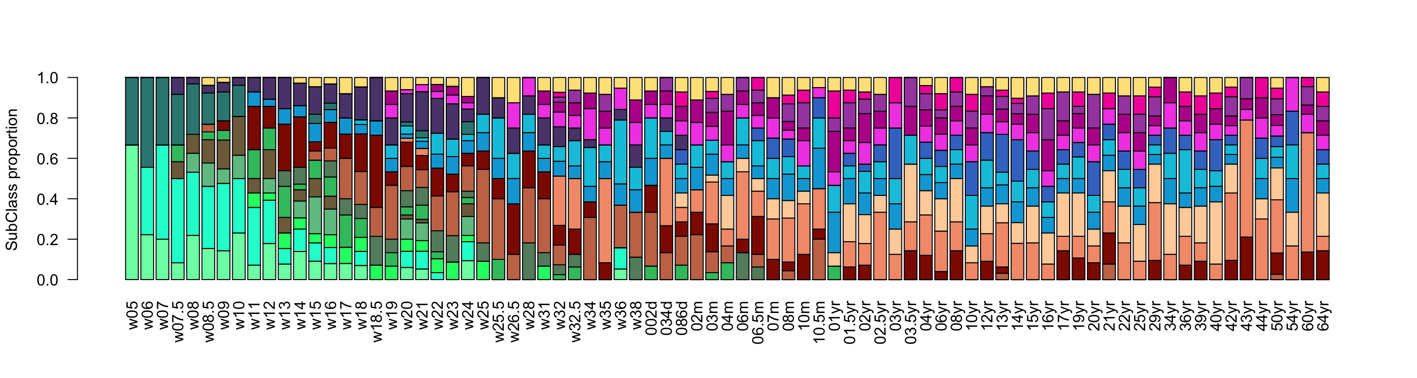

Figure 2.12: Corticogenesis subclasses proportions.

Increasing the resolution and going to the neuron-specific network, we can observe that progenitors start to decrease around the neurogenesis peak (w14-16), and mature neurons are predominant postnatally. Furthermore, the defined neuronal subclasses depict the inside-out stereotypical way of cortical development. Deep non intratelencephalic (Non-IT) are followed by intratelencephalic (IT) ones, with the upper layer IT neurons (ExN-L2-3-IT) being the last to mature.

barplot(neurogenesis_subclass_proportion[,ordered_ages], 
        col = neurogenesis_palette[rownames(neurogenesis_subclass_proportion)], 
        las = 2, 
        ylab = 'SubClass proportion')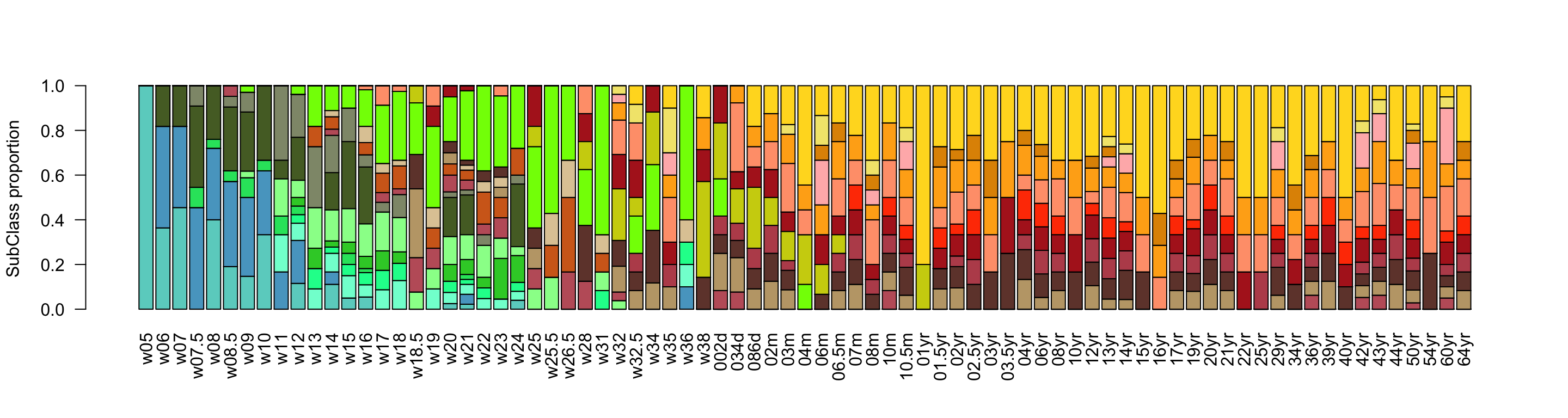

Figure 2.13: Neurogenesis subclasses proportions.

In the gliogenesis network, instead, we identified more progenitor subclasses. In early stages we can observe a variety of radial glia, with a nice distinction between different cell cycle phases (G2M and S). In time progenitors associated to later stages of development appear, such as oRG and tRG. Gliogenesis comprises two major differentiation trajectories: astrogenesis and oligodendrogenesis. Cell types of these two branches appear already between w10 and w18. Early OPCs coming from the ganglionic eminences migrate towards the cortex, temporally followed by cortical radial glia generating astrocytes after neurogenesis (peak w18-w25).

barplot(gliogenesis_subclass_proportion[,ordered_ages[which(ordered_ages %in% colnames(gliogenesis_subclass_proportion))]],
        col = gliogenesis_palette[rownames(gliogenesis_subclass_proportion)], 
        las = 2, 
        ylab = 'SubClass proportion')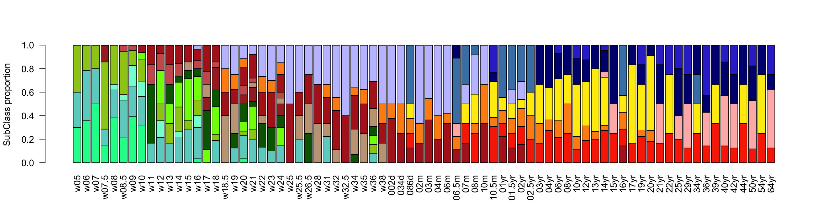

Figure 2.14: Gliogenesis Subclasses proportions.

2.5.2 Compute the cumulative cluster number proportion

Another way of looking cell type dynamics during cortical development involves examining the number of clusters assigned to each subtype across developmental stages.

Show the code (subtype cumulative sum by lineage)

# here for each row (i.e. for each subclass/subtype) 
# ordered by age, we divide the cumulative sum of 
# clusters by the total number of clusters to obtain 
# subclass/subtype proportion for each stage

corticogenesis_subclass_cumsum <- t(
  apply(X = table(corticogenesis_sce$SubClass, corticogenesis_sce$Stages)[,mixedsort(unique(corticogenesis_sce$Stages))],  
        MARGIN =  1, 
        FUN = function(i) {
  cumsum(i/sum(i)) 
})) 

neurogenesis_subclass_cumsum <- t(apply(table(neurogenesis_sce$SubClass, neurogenesis_sce$Stages)[,mixedsort(unique(neurogenesis_sce$Stages))], 1, function(i) {
  cumsum(i/sum(i))
}))

gliogenesis_subclass_cumsum <- t(apply(table(gliogenesis_sce$SubClass, gliogenesis_sce$Stages)[,mixedsort(unique(gliogenesis_sce$Stages))], 1, function(i) {
  cumsum(i/sum(i))
}))

The cumulative sum gives us different levels of information. First, we can observe the time point in which a cell type starts to populate the cortex; second, we can see when the proportion of clusters increases the fastest, showing a prevalence of generation or maturation of the subclasses; third, we can appreciate the period of time in which each cell type reaches its plateau, i.e. is not generated anymore or has fully matured. For example, radial glia reach their plateau before birth, similarly to immature inhibitory neurons, which in time leave place to mature inhibitory neurons. Oligodendrocytes, instead, appear postnatally with a peak around late childhood and only reach their plateau in adulthood, in accordance with the processes of synaptogenesis and myelination.

Show the code (plotting corticogenesis)

par(mar=c(4.2,3,1,1))
plot(corticogenesis_subclass_cumsum[1,], 
     type = 'l',
     las = 1,
     lwd = 2, 
     col = corticogenesis_palette[rownames(corticogenesis_subclass_cumsum)[1]], 
     xlab = 'Stage', 
     ylab = 'Cumulative cluster proportion', 
     ylim = c(min(corticogenesis_subclass_cumsum), max(corticogenesis_subclass_cumsum)),
     xaxt="n")
axis(side = 1, 
     labels = stages.indexes,
     at = 1:length(stages.indexes),
     las = 1)
for(i in seq(2, nrow(corticogenesis_subclass_cumsum))) {
  lines(corticogenesis_subclass_cumsum[i,], 
        las = 1,
        lwd = 2.5, 
        col = corticogenesis_palette[rownames(corticogenesis_subclass_cumsum)[i]])
}

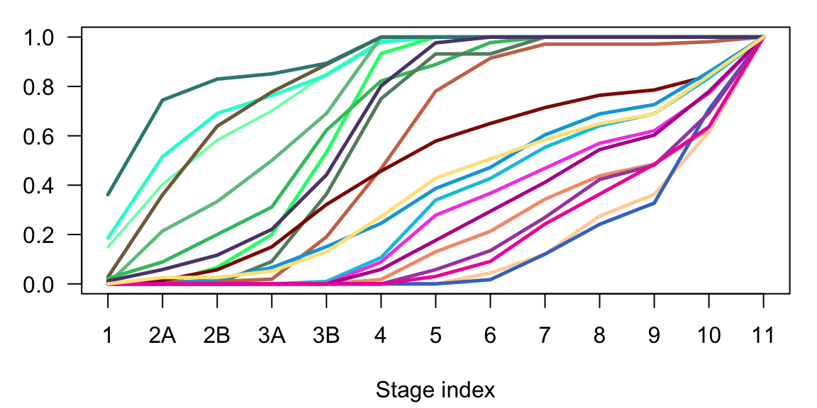
Figure 2.15: Corticogenesis cumulative sum of subclasses cells in time.

In neurogenesis the most evident difference is between the maturing and the differentiated excitatory neurons subclasses. Moreover, it is evident the difference between deep and upper layer neurons, and particularly between the non intratelencephalic (Non-IT) and the intratelencephalic (IT) branches.

Show the code (plotting neurogenesis)

par(mar=c(4.2,3,1,1))
plot(neurogenesis_subclass_cumsum[1,], 
     type = 'l', 
     las = 1,
     lwd = 2, 
     col = neurogenesis_palette[rownames(neurogenesis_subclass_cumsum)[1]], 
     xlab = 'Stage index', 
     ylab = 'Cumulative cluster proportion', 
     ylim = c(min(neurogenesis_subclass_cumsum), max(neurogenesis_subclass_cumsum)),
     xaxt="n")
axis(side = 1, 
     labels = stages.indexes,
     at = 1:length(stages.indexes),
     las = 1)
for(i in seq(2, nrow(neurogenesis_subclass_cumsum))) {
  lines(neurogenesis_subclass_cumsum[i,], 
        lwd = 2.5, 
        col = neurogenesis_palette[rownames(neurogenesis_subclass_cumsum)[i]])
}

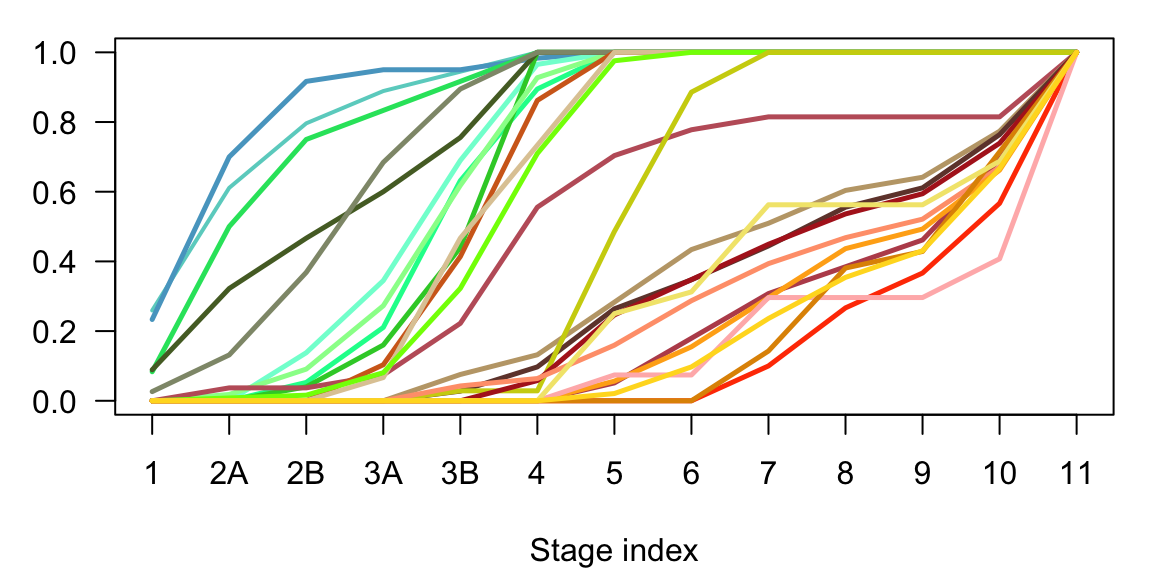
Figure 2.16: Neurogenesis cumulative sum of subclasses cells in time.

In gliogenesis the main difference is between progenitors (radial glia and OPCs), and the mature cell types (oligodendrocytes and astrocytes).

Show the code (plotting gliogenesis)

par(mar=c(4.2,3,1,1))
plot(gliogenesis_subclass_cumsum[1,], 
     type = 'l',
     las = 1,
     lwd = 2.5, 
     col = gliogenesis_palette[rownames(gliogenesis_subclass_cumsum)[1]], 
     xlab = 'Stage index', 
     ylab = 'Cumulative cluster proportion', 
     ylim = c(min(gliogenesis_subclass_cumsum), max(gliogenesis_subclass_cumsum)),
     xaxt="n")
axis(side = 1, 
     labels = stages.indexes,
     at = 1:length(stages.indexes),
     las = 1)
for(i in seq(2, nrow(gliogenesis_subclass_cumsum))) {
  lines(gliogenesis_subclass_cumsum[i,], 
        lwd = 2, 
        col = gliogenesis_palette[rownames(gliogenesis_subclass_cumsum)[i]])
}

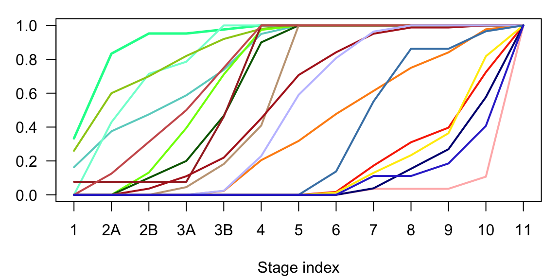
Figure 2.17: Gliogenesis cumulative sum of subclasses cells in time.

2.6 Stages composition across subclasses

To follow the stage composition among the different subclasses, we can look at the proportion of clusters of each age within the identified subclasses. We can first order them by mean age, and then calculate stages fractions.

Show the code (ordering age)

cortico_mean_age <- unlist(lapply(unique(corticogenesis_sce$SubClass), function(i) {
  subclass_days <- corticogenesis_sce$Days[which(corticogenesis_sce$SubClass == i)]
  log_subclass_days <- log10(subclass_days)
  mean_age <- mean(log_subclass_days)
}))
names(cortico_mean_age) <- unique(corticogenesis_sce$SubClass)

neuro_mean_age <- unlist(lapply(unique(neurogenesis_sce$SubClass), function(i) {
  subclass_days <- neurogenesis_sce$Days[which(neurogenesis_sce$SubClass == i)]
  log_subclass_days <- log10(subclass_days)
  mean_age <- mean(log_subclass_days)
}))
names(neuro_mean_age) <- unique(neurogenesis_sce$SubClass)

glio_mean_age <- unlist(lapply(unique(gliogenesis_sce$SubClass), function(i) {
  subclass_days <- gliogenesis_sce$Days[which(gliogenesis_sce$SubClass == i)]
  log_subclass_days <- log10(subclass_days)
  mean_age <- mean(log_subclass_days)
}))
names(glio_mean_age) <- unique(gliogenesis_sce$SubClass)

Show the code (stages proportion in subclasses)

corticogenesis_stage_proportion <- table(corticogenesis_sce$Stages, 
                                         corticogenesis_sce$SubClass)

corticogenesis_stage_proportion <- t(t(corticogenesis_stage_proportion)/colSums(corticogenesis_stage_proportion))


neurogenesis_stage_proportion <- table(neurogenesis_sce$Stages, 
                                       neurogenesis_sce$SubClass)

neurogenesis_stage_proportion <- t(t(neurogenesis_stage_proportion)/colSums(neurogenesis_stage_proportion))


gliogenesis_stage_proportion <- table(gliogenesis_sce$Stages, 
                                      gliogenesis_sce$SubClass)

gliogenesis_stage_proportion <- t(t(gliogenesis_stage_proportion)/colSums(gliogenesis_stage_proportion))

barplot(corticogenesis_stage_proportion[,names(cortico_mean_age[order(cortico_mean_age)])],
        col = stages_palette[rownames(corticogenesis_stage_proportion)], 
        las = 2, 
        ylab = 'Stages proportion')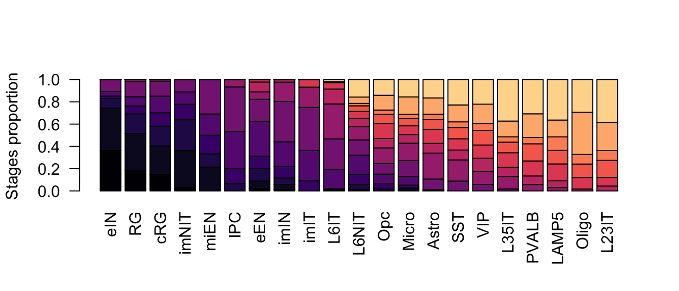

Figure 2.18: Corticogenesis subclasses proportions.

barplot(neurogenesis_stage_proportion[,names(neuro_mean_age[order(neuro_mean_age)])],
        col = stages_palette[rownames(neurogenesis_stage_proportion)], 
        las = 2, 
        ylab = 'Stages proportion')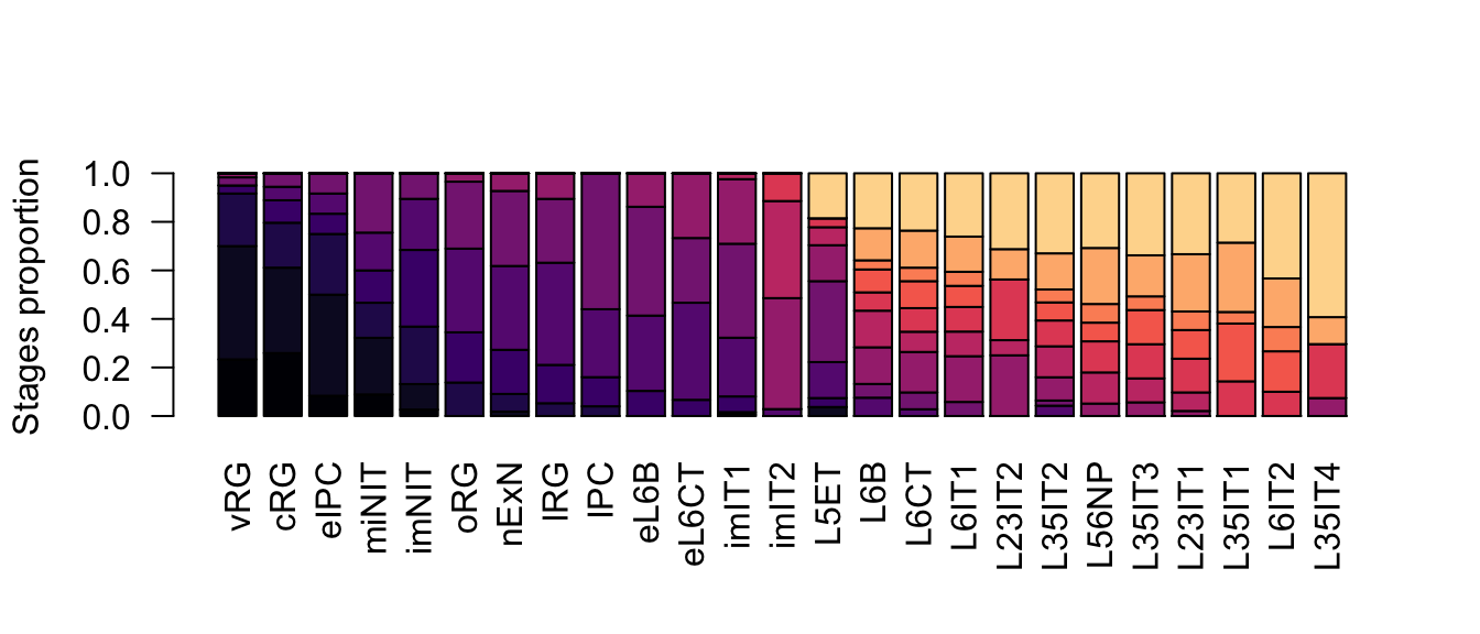

Figure 2.19: Neurogenesis subclasses proportions.

barplot(gliogenesis_stage_proportion[,names(glio_mean_age[order(glio_mean_age)])],
        col = stages_palette[rownames(gliogenesis_stage_proportion)], 
        las = 2, 
        ylab = 'Stages proportion')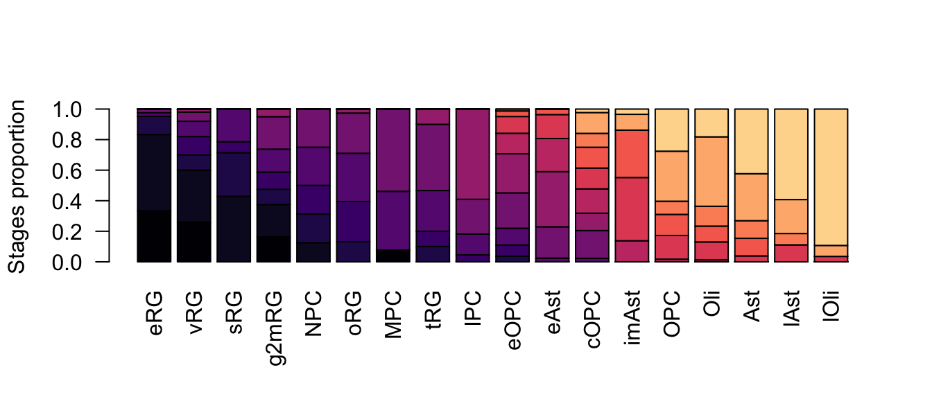

Figure 2.20: Gliogenesis subclasses proportions.

1 Summary

3 Analysis Tools