5 Mapping Single-cell data
5.1 Quickstart
These are the main functions to map a single-cell RNA-sequencing dataset on the corticogenesis resource. This implies that the data loaded are already cluster profiles (or pseudobulk). Below we will report a detailed description and examples on how to compute cluster profiles and perform mapping and further related analyses.
#STEP 1: load libraries
library(neuRoDev)

#STEP 2: load data
corticogenesis_sce <- corticogenesis.sce(directory = '~/Downloads')
data <- readRDS('my_data') #choose your data object

#STEP 3: mapping
mapped_sc_pseudo <- mapNetwork(net = corticogenesis_sce,
                               new_profiles = data)

#STEP 4: inspect mapping
mapped_sc_pseudo$new_plot
mapped_sc_pseudo$annotation$Barplot
mapped_sc_pseudo$annotation$Best.Annotation
5.2 Loading necessary libraries and data
5.2.2 Loading the networks necessary objects
corticogenesis_sce <- corticogenesis.sce(directory = '~/Downloads')
neurogenesis_sce <- neurogenesis.sce(directory = '~/Downloads')
gliogenesis_sce <- gliogenesis.sce(directory = '~/Downloads')
5.3 Mapping a single cell RNAseq dataset
5.3.1 Data preprocessing
This example dataset from Kanton et al. (2019) can be downloaded here (ExtraData_Tutorial folder). For the scope of the analyses, we pre-processed the data, removing low quality cells. We also performed proportional random sampling to ease following this tutorial, to a total of 10.000 cells. This implies the reduction of total cell number while keeping cell groups proportions.
To reproduce the figures in the paper, we used the complete dataset, processed using the ACTIONet pipeline up to clustering (see: ACTIONet Tutorial. The data were processed by using the following functions with default parameters: normalize.ace, reduce.ace, runACTIONet, clusterCells).
Warning: quality control needs to be done specifically to your dataset. We assume that cells in the following steps have passed standard quality controls. You can refer to the Seurat pipeline or to the scanpy pipeline in Python.
ext_count_matrix <- readRDS('~/Downloads/sc_count_matrix.rds')Here we report the detailed pipeline of the standard Seurat steps required to obtain clusters, which are needed for the following analyses. It is possible to customize some parameters for the pipeline, which have to be tuned to your specific dataset.
Show code
# The pre-processing steps are done following the standard Seurat pipeline:
library(Seurat)

sc_seu <- CreateSeuratObject(counts = ext_count_matrix)
sc_seu <- NormalizeData(object = sc_seu)
sc_seu <- FindVariableFeatures(object = sc_seu, span = 0.3)
sc_seu <- ScaleData(object = sc_seu, features = VariableFeatures(sc_seu))
numPCs <- min(50, ncol(ext_count_matrix) - 1)
sc_seu <- RunPCA(object = sc_seu, features = VariableFeatures(sc_seu), npcs = numPCs, approx = FALSE)

PCs_to_use <- (sc_seu$pca@stdev)^2
PCs_to_use <- PCs_to_use/sum(PCs_to_use)
PCs_to_use <- cumsum(PCs_to_use)
PCs_to_use <- min(which(PCs_to_use >= 0.75))

PCs_to_use <- min(numPCs, PCs_to_use)

sc_seu <- FindNeighbors(object = sc_seu, dims = seq_len(PCs_to_use))
sc_seu <- FindClusters(object = sc_seu, resolution = 1, algorithm = 4, random.seed = 1) # if this gives an error, try setting algorithm to 1 or check ?FindClusters

sc_seu <- RunUMAP(sc_seu, dims = seq_len(PCs_to_use))
We can then visualize the UMAP with the clusters:
DimPlot(sc_seu,
        reduction = "umap",
        label = TRUE)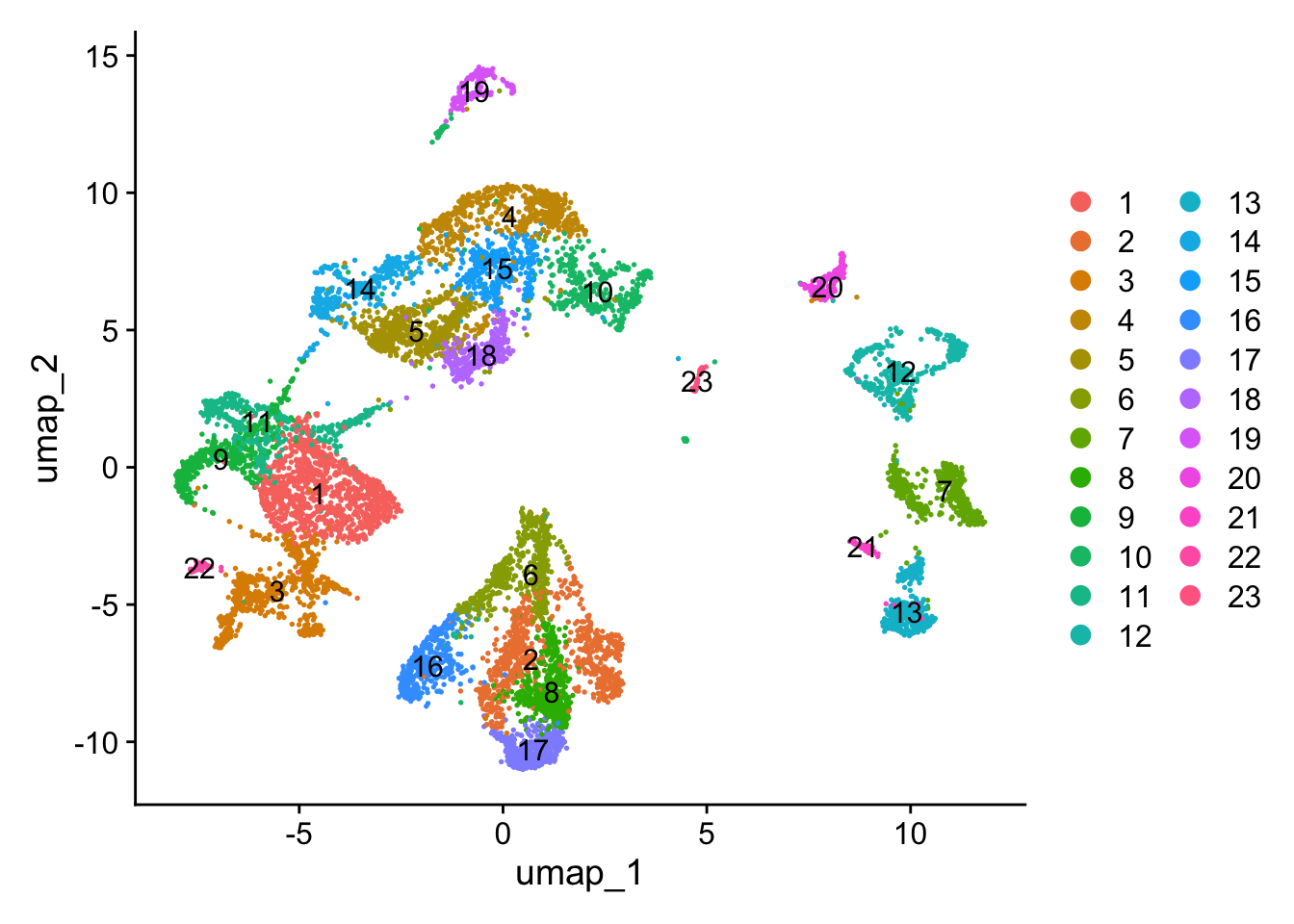
Figure 5.1: Single-cell dataset UMAP with clusters.
Since this dataset contains cells from different stages, we can also check the stages distribution and map this information on the single cells:
stage_annotation <- unlist(lapply(strsplit(colnames(sc_seu), '.', fixed = TRUE), function(i) {i[2]}))
names(stage_annotation) <- Cells(sc_seu)

sc_seu$stage <- stage_annotation

stages_palette <- viridis(n = length(unique(stage_annotation)))
names(stages_palette) <- unique(stage_annotation)

DimPlot(
  sc_seu,
  group.by = "stage",
  reduction = "umap",
  cols = stages_palette
)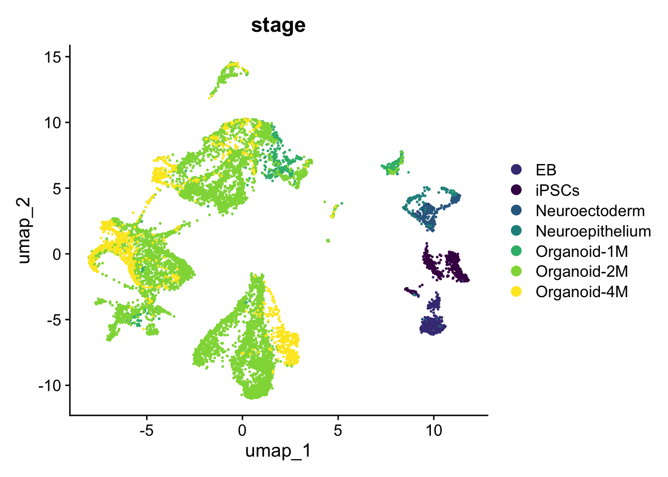
Figure 5.2: Single-cell dataset UMAP colored by stage.
5.3.2 Data summary
The standard mapping procedure requires the definition of summary transcriptional profiles for each cluster, that can be obtained in two ways:
- Pseudobulk profiles (obtained by summing all counts in a cluster together and then normalizing using Counts Per Million (CPM)).
- Expression signatures (obtained by averaging the normalized counts of all cells in a cluster and then subtracting the mean expression across all cells).
Depending on the type of question, the user can choose the most suitable summary profile. The key distinction lies in the type of information captured: signatures represent relative expression, describing how a given cluster differs from the others and thus highlighting differences. In contrast, pseudobulk profiles capture absolute expression levels and are therefore more suitable for biological interpretation without emphasizing relative changes. Signatures are not suited if used in a relatively homogeneous dataset, as they will greatly enhance subtle differences which may just depict noise. For the following example we will use the most straightforward approach by mapping pseudobulk profiles.
Pseudobulk profiles can be computed using the get_pseudobulk function, which will save as a SingleCellExperiment object the pseudobulk counts in counts and the log-normalized Counts Per Million in logcounts
We now define the pseudobulks of the clusters that we obtained following the Seurat pipeline:
sc_pseudo <- get_pseudobulk(exp_matrix = sc_seu@assays$RNA$counts,
                            membership_vector = sc_seu$seurat_clusters)
colnames(sc_pseudo) <- paste0('c', colnames(sc_pseudo)) #to have strings and not numbers
5.3.3 Mapping on the reference network
Now comes the actual mapping part, which can be easily performed using the mapNetwork function, that requires the following main inputs:
-
net= the reference network to use. -
new_profiles= the transcriptional profiles to map (either pseudobulk or signatures).
Other useful inputs can be checked in the function help (?mapNetwork).
Since in the original paper they mention the presence of glial cell types, as well as inhibitory and excitatory neurons, it is reasonable to map on the corticogenesis network. If your experimental design already defines the presence of only glial cells or only excitatory neurons (with their respective precursors), then it is suggested to map only on the neurogenesis and gliogenesis steps. Another approach is to first map on the more general corticogenesis network and then map again on the precise lineage-specific networks, also on a subset of cells.
mapped_sc_pseudo <- mapNetwork(net = corticogenesis_sce,
                               new_profiles = logcounts(sc_pseudo))
We can now visualize the network with the mapped clusters on top:
mapped_sc_pseudo$new_plot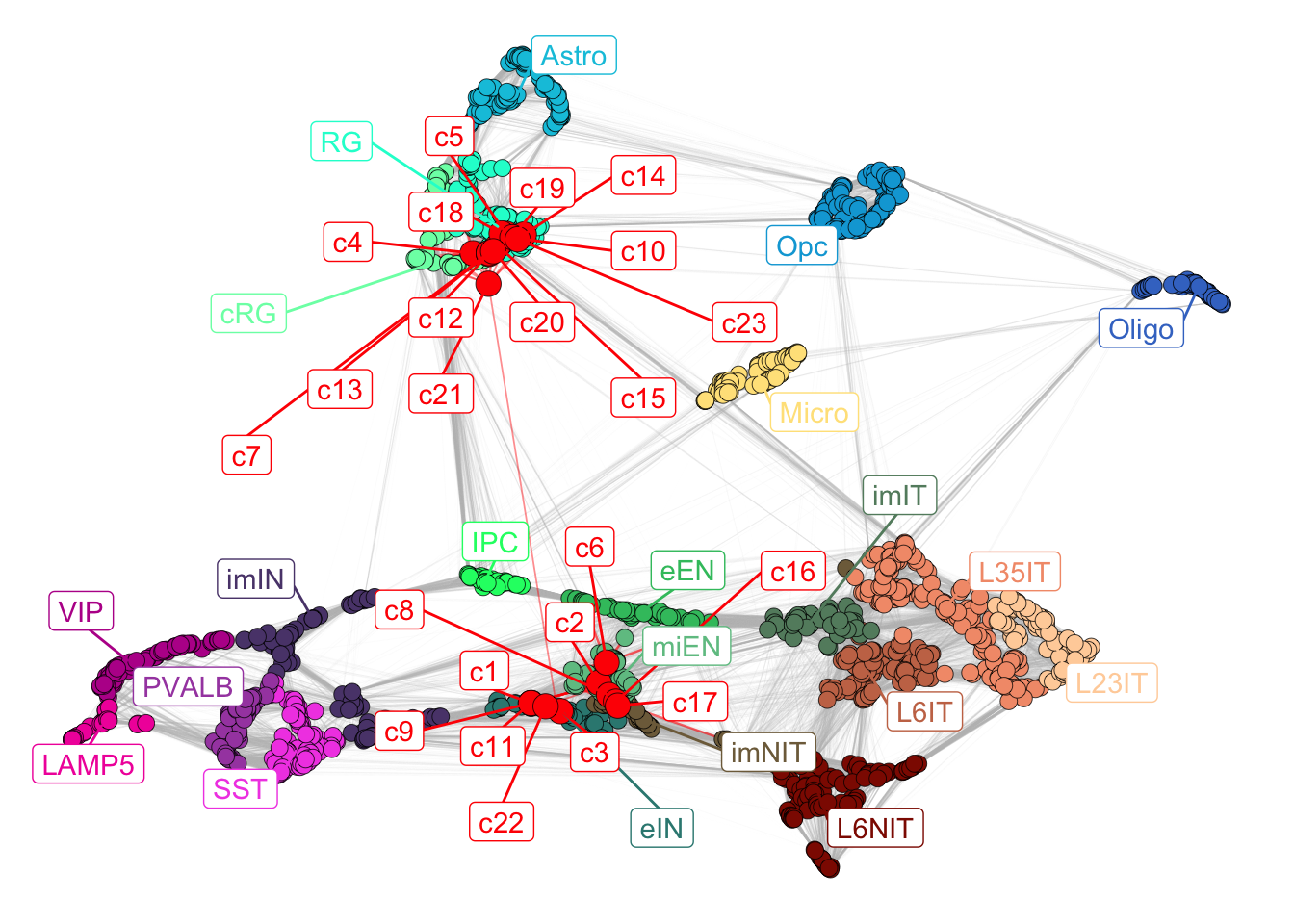
Figure 5.3: Corticogenesis network with mapped clusters.
Newly mapped clusters will locate close to the most similar reference clusters, so it is possible to observe the most similar subclasses for each mapped cluster.
By visualizing the mapped network, we can already appreciate how the clusters generally map into two different sections of the network, one close to radial glia and cycling radial glia, while the other close to immature neurons. To quantify similarity, we developed a score per subclass per cluster, using the 15 most similar reference clusters’ annotations (the number of reference clusters to use can be set by changing n_nearest in the mapNetwork function).
This score sums up to 1 and represents the weighted fraction of clusters in the neighborhood belonging to the different subclasses.
The score can be visualized with a barplot reporting the proportions (between 0-1) of the different subclasses across the mapped clusters.
mapped_sc_pseudo$annotation$Barplot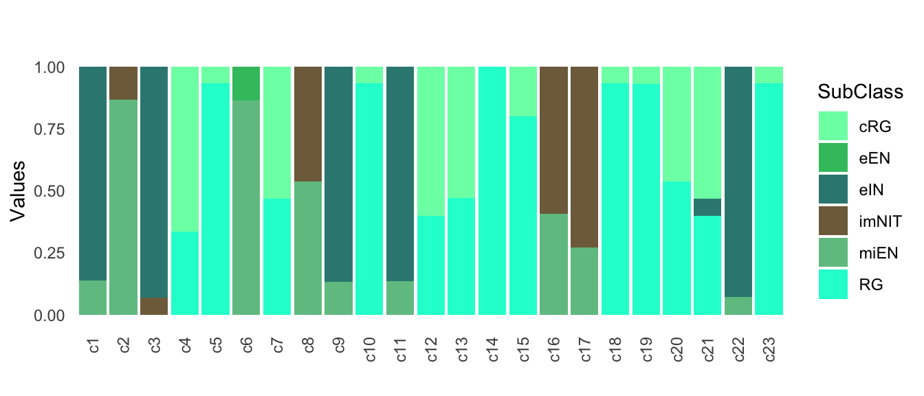
Figure 5.4: Annotation scores across clusters.
To get a single label for each mapped cluster, we take the maximum of these scores. This depicts the most similar subclass among the closest neighbors.
mapped_sc_pseudo$annotation$Best.Annotation
#>      c1      c2      c3      c4      c5      c6      c7
#>   "eIN"  "miEN"   "eIN"   "cRG"    "RG"  "miEN"   "cRG"
#>      c8      c9     c10     c11     c12     c13     c14
#>  "miEN"   "eIN"    "RG"   "eIN"   "cRG"   "cRG"    "RG"
#>     c15     c16     c17     c18     c19     c20     c21
#>    "RG" "imNIT" "imNIT"    "RG"    "RG"    "RG"   "cRG"
#>     c22     c23
#>   "eIN"    "RG"
The same quantification can be obtained for stages of maturation, either by specifying color_attr = 'Stages' in the mapNetwork function, or by running the annotateMapping function, which requires the following inputs:
-
net= the reference network to use. -
new_cor= the correlation between mapped points and reference clusters, which can be found inmapped_object$new_cor. -
color_attr= the annotation label to use, in this case ‘Stages’.
Our mapping strategy allows the mapping of any expression matrix, thus we added a quantification of the mapping confidence, described with two diverse measures:
confidence (
mapped_object$annotation$Mapping.Confidence) for each mapped point, showing the average of the 15 highest correlation values that the mapped point has with the reference clusters.global confidence (
mapped_object$annotation$Global.Confidence), describing the average confidence across all mapped point.
The confidence values can be accessed in the following way:
# per cluster confidence
mapped_sc_pseudo$annotation$Mapping.Confidence
#>        c1        c2        c3        c4        c5        c6
#> 0.7130546 0.7547882 0.6901726 0.8477842 0.7965150 0.7947670
#>        c7        c8        c9       c10       c11       c12
#> 0.6281157 0.7647813 0.7314415 0.7639241 0.7194806 0.6995298
#>       c13       c14       c15       c16       c17       c18
#> 0.6288900 0.7215679 0.8474292 0.7706888 0.7342306 0.8037366
#>       c19       c20       c21       c22       c23
#> 0.6317051 0.7253773 0.5659153 0.6400742 0.5006500

# global confidence
mapped_sc_pseudo$annotation$Global.Confidence
#> [1] 0.7162878
The confidence score not only tells how similar are the mapped points to neighboring clusters, but also can help identifying profiles of low quality or cells of cell types not represented in the resource.
For example, cluster 23 has a slightly lower confidence score (~0.50) compared to the others, so it may be worth further checking the quality of the cells in that cluster (not done here), to assess whether this could be a low quality group of cells.
Sometimes clusters have a high confidence score, but neighbors with different annotations, making it hard to actually infer a single annotation. To help with this, it is possible to apply the confidence score to the inferred annotations defined above:
# checking the annotation confidence of the first five clusters
mapped_sc_pseudo$annotation$Annotations.Confidence[seq(1,5)]
#> $c1
#>        eIN       miEN
#> 0.61520448 0.09785007
#>
#> $c2
#>      miEN     imNIT
#> 0.6538900 0.1008981
#>
#> $c3
#>        eIN      imNIT
#> 0.64261159 0.04756101
#>
#> $c4
#>       cRG        RG
#> 0.5631011 0.2846830
#>
#> $c5
#>         RG        cRG
#> 0.74243175 0.05408324
5.3.4 Knowledge transfer
The annotations newly defined can now be transferred to the original dataset and visualized at the single cell level.
new_annotation <- mapped_sc_pseudo$annotation$Best.Annotation[paste0('c', sc_seu$seurat_clusters)]
names(new_annotation) <- Cells(sc_seu)

sc_seu$annotation <- new_annotation

corticogenesis_palette <- unique(corticogenesis_sce$SubClass_color)
names(corticogenesis_palette) <- unique(corticogenesis_sce$SubClass)


DimPlot(
  sc_seu,
  reduction = "umap",
  label = TRUE,
) +
  ggtitle("clusters") +
  theme(plot.title = element_text(hjust = 0.5))

DimPlot(
  sc_seu,
  group.by = "annotation",
  reduction = "umap",
  cols = corticogenesis_palette,
  label = TRUE,
) +
  ggtitle("annotation") +
  theme(plot.title = element_text(hjust = 0.5))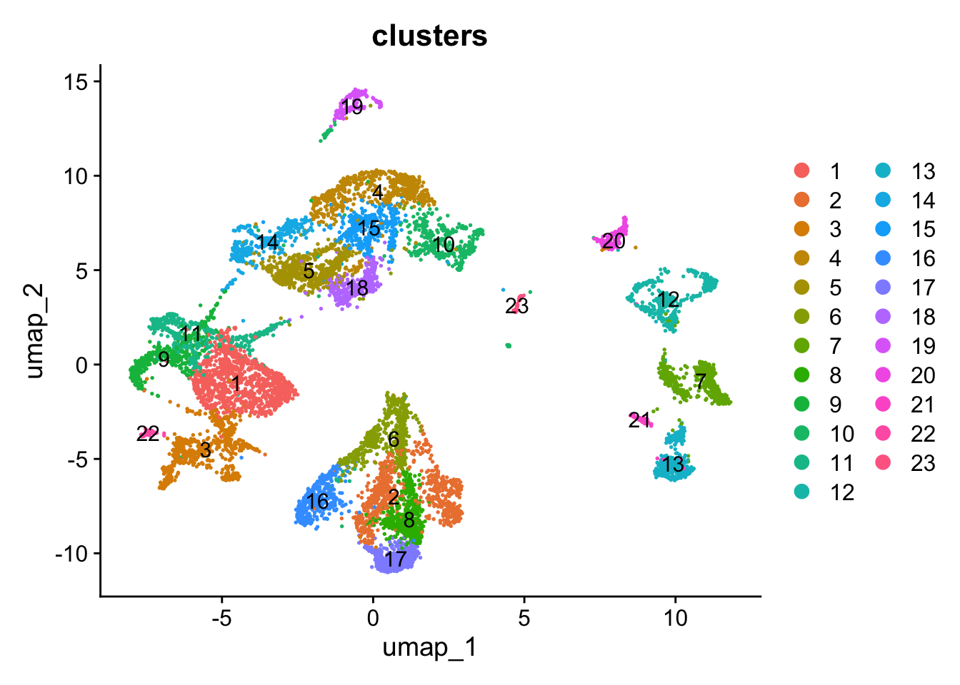
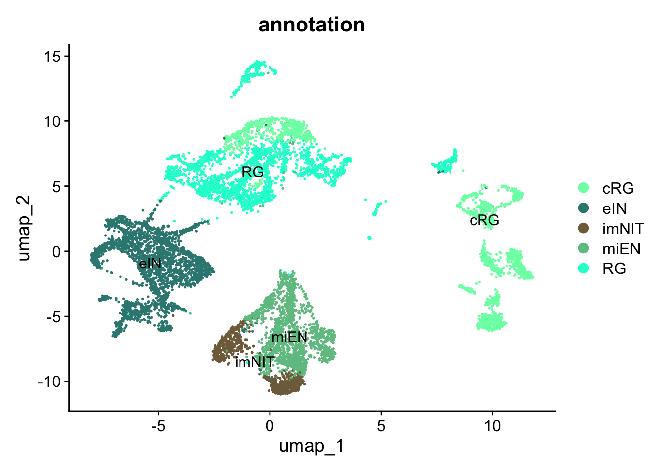
Figure 5.5: Single-cell dataset UMAP with clusters and annotations.
By looking at the UMAP labelled by cluster together with the newly annotated UMAP, we can appreciate that the cells annotated as cRG that are close to all the cells annotated as RG are indeed those of the cluster 4, the cluster with similar annotation values for both cRG and RG.
To further validate the annotation, we can also visualize the preferentially expressed genes in the relevant subclasses. We report gene sets preferentially expressed in each reference subclass or subclass group here (PreferentialExpression folder).
corticogenesis_pe_genes <- readRDS("~/Downloads/corticogenesis_subclass_preferential_genes.rds")
neurogenesis_pe_genes <- readRDS("~/Downloads/neurogenesis_subclass_preferential_genes.rds")
gliogenesis_pe_genes <- readRDS("~/Downloads/gliogenesis_subclass_preferential_genes.rds")
We can compute for the annotations of interest the mean expression of preferential genes in the single-cell dataset.
sc_seu$eIN.Score <- Matrix::colMeans(
  GetAssayData(sc_seu, layer = "data")[corticogenesis_pe_genes$eIN[which(corticogenesis_pe_genes$eIN %in% rownames(sc_seu))],])


sc_seu$cRG.Score <- Matrix::colMeans(
  GetAssayData(sc_seu, layer = "data")[corticogenesis_pe_genes$cRG[which(corticogenesis_pe_genes$cRG %in% rownames(sc_seu))],])


sc_seu$RG.Score <- Matrix::colMeans(
  GetAssayData(sc_seu, layer = "data")[corticogenesis_pe_genes$RG[which(corticogenesis_pe_genes$RG %in% rownames(sc_seu))],])


sc_seu$imNIT.Score <- Matrix::colMeans(
  GetAssayData(sc_seu, layer = "data")[corticogenesis_pe_genes$imNIT[which(corticogenesis_pe_genes$imNIT %in% rownames(sc_seu))],])


sc_seu$miEN.Score <- Matrix::colMeans(
  GetAssayData(sc_seu, layer = "data")[corticogenesis_pe_genes$miEN[which(corticogenesis_pe_genes$miEN %in% rownames(sc_seu))],])
FeaturePlot(sc_seu,
            features = "eIN.Score",
            reduction = "umap") + ggtitle("eIN")
FeaturePlot(sc_seu,
            features = "cRG.Score",
            reduction = "umap") + ggtitle("cRG")
FeaturePlot(sc_seu,
            features = "RG.Score",
            reduction = "umap") + ggtitle("RG")
FeaturePlot(sc_seu,
            features = "imNIT.Score",
            reduction = "umap") + ggtitle("imNIT")
FeaturePlot(sc_seu,
            features = "miEN.Score",
            reduction = "umap") + ggtitle("miEN")
DimPlot(
  sc_seu,
  reduction = "umap",
  group.by = "annotation",
  cols = corticogenesis_palette,
  label = TRUE,
) +
  ggtitle("annotation") +
  theme(plot.title = element_text(hjust = 0.5))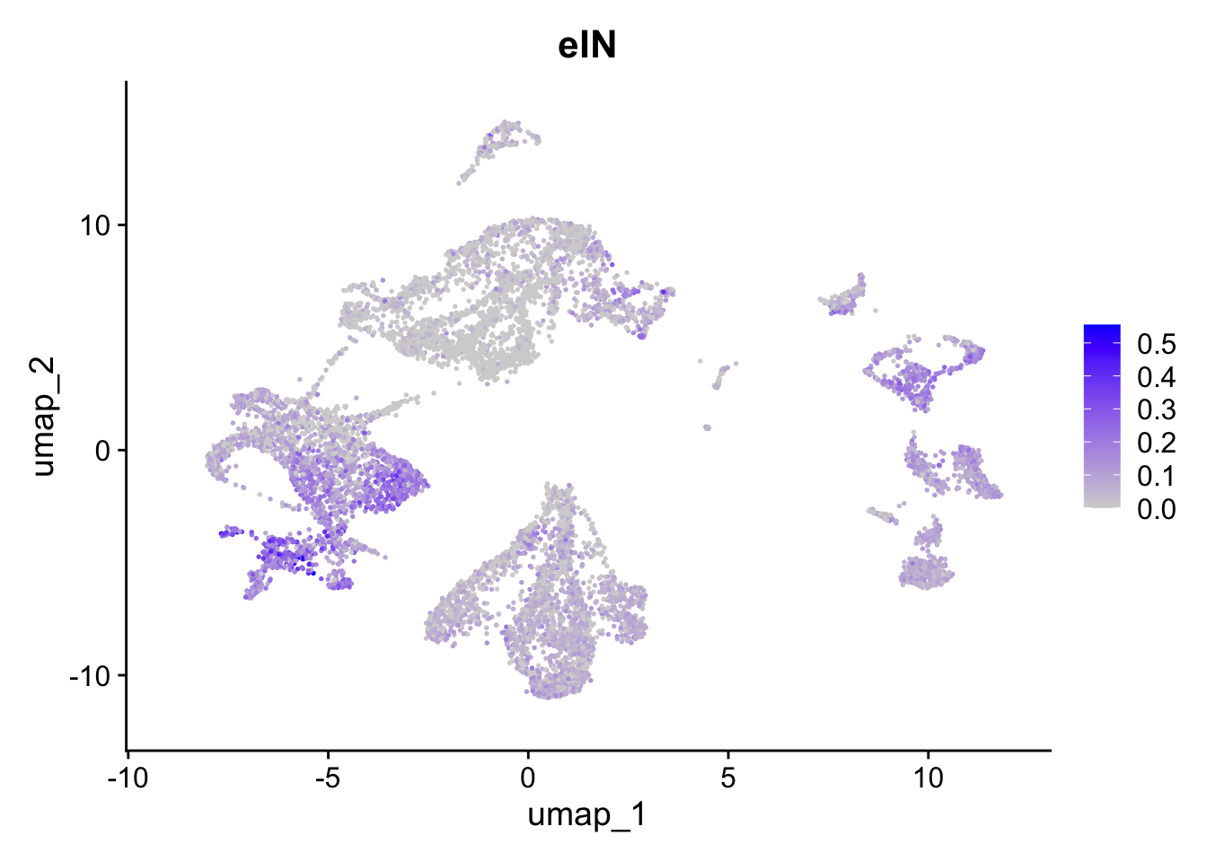
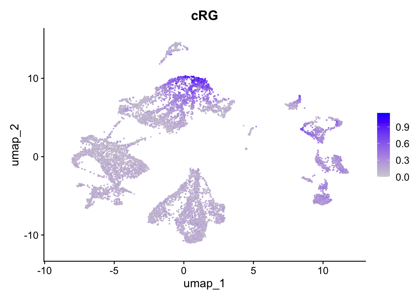
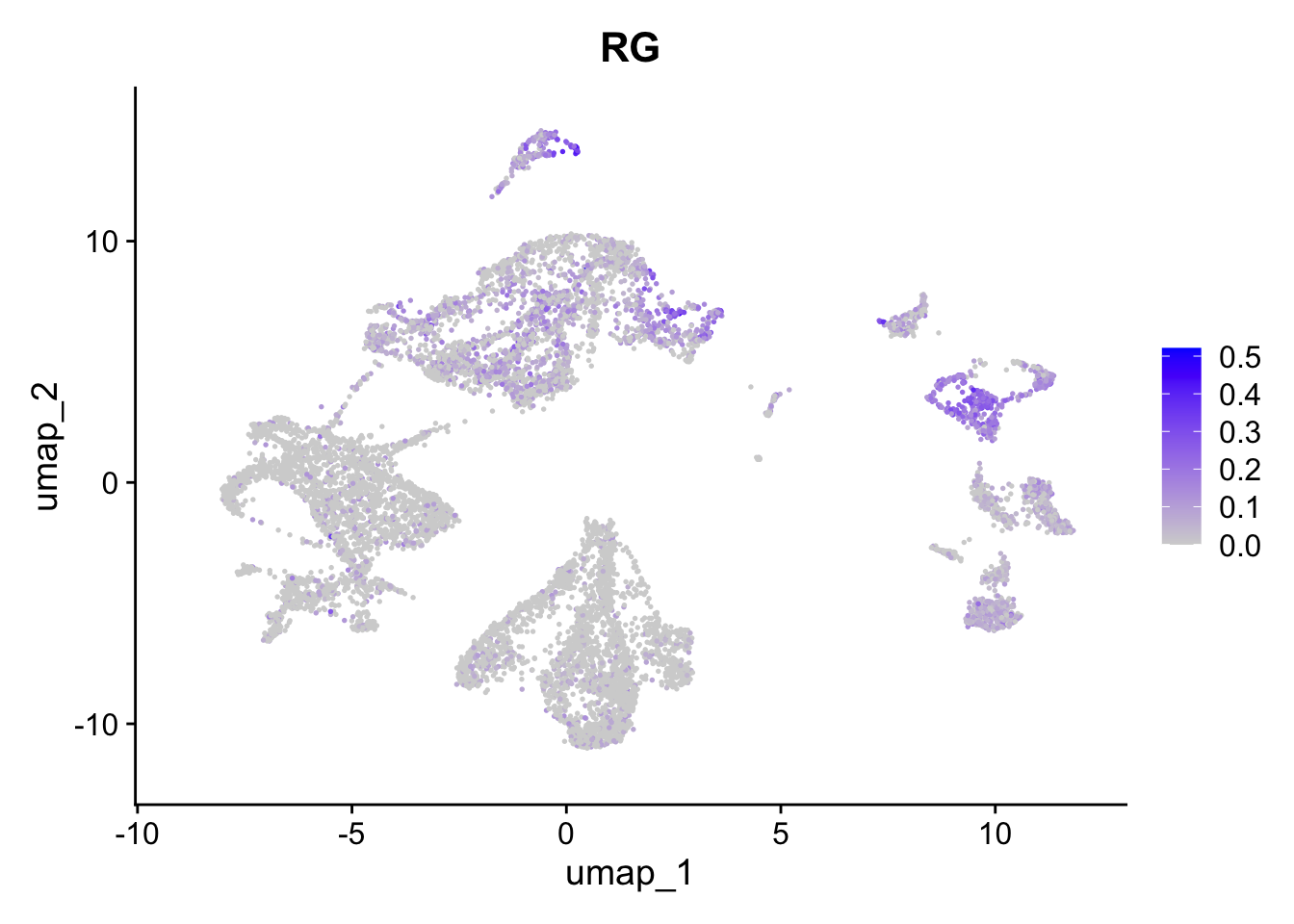
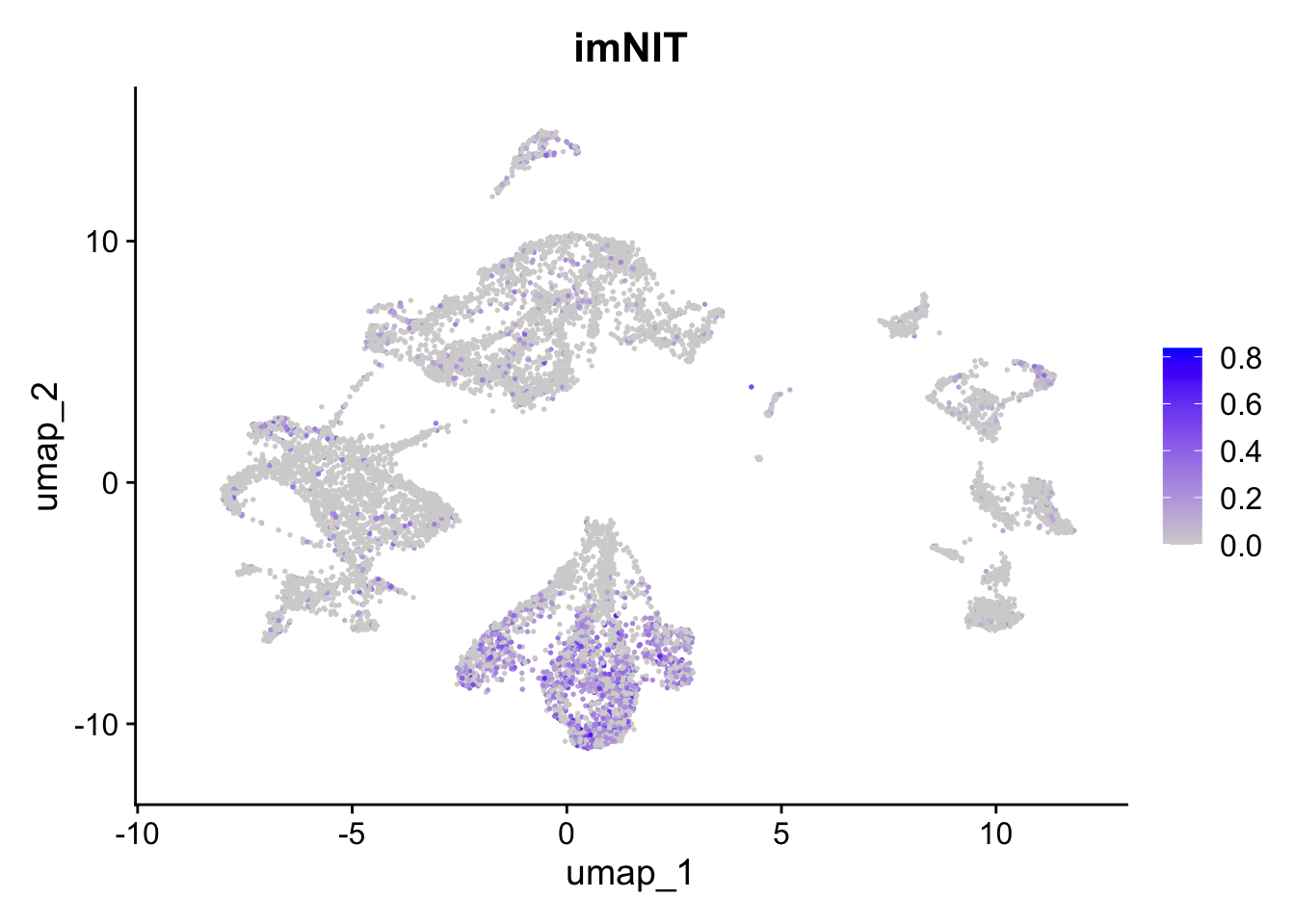
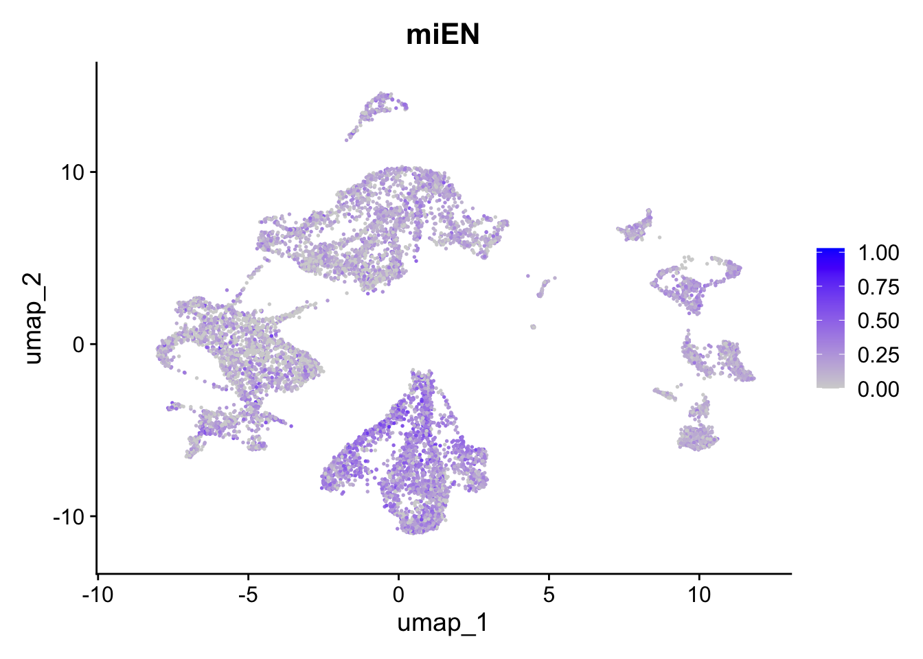

Figure 5.6: Preferential genes expression
The expression of preferentially expressed genes defined in our resource match the assigned labels, confirming the annotations given by the mapping strategy. To further characterize our clusters, we can leverage the list of our manually curated Gene Ontology Biological Processes for the corticogenesis and neurogenesis networks and assess their expression levels in the mapped clusters. The list of manually curated Biological Processes can be downloaded from here (PreferentialExpression folder).
corticogenesis_GO <- readRDS('~/Downloads/corticogenesis_GOBP_genesets.rds')
neurogenesis_GO <- readRDS('~/Downloads/neurogenesis_GOBP_genesets.rds')
The preferential expression values of Gene Ontology Biological Processes (BP), Molecular Functions (MF), and Cellular Components (CC) for the three reference networks is also provided in the resource, and is available here (PreferentialExpression folder).
Each object is a list containing preferential expression scores in one of the three reference networks in the three ontologies (BP, MF, CC). Each element of each list contains the activity (activity) derived from Gene Set Variation Analysis (one value per gene set in each cluster) and the preferential expression scores (preferential; one value per gene set in each subclass).
corticogenesis_preferential_GO <- readRDS('~/Downloads/corticogenesis_preferential_GO.rds')
neurogenesis_preferential_GO <- readRDS('~/Downloads/neurogenesis_preferential_GO.rds')
gliogenesis_preferential_GO <- readRDS('~/Downloads/gliogenesis_preferential_GO.rds')
First, we compute the average expression of those gene sets:
sc_seu_cortico_GOBP <- do.call(rbind, lapply(corticogenesis_GO, function(g) {

  g <- g[which(g %in% rownames(sc_seu))]

  Matrix::colMeans(logcounts(sc_pseudo)[g,])

}))

rownames(sc_seu_cortico_GOBP) <- gsub(" \\(GO:[0-9]+\\)$", "", rownames(sc_seu_cortico_GOBP)) #to simplify the gene sets names

sc_seu_cortico_GOBP <- sc_seu_cortico_GOBP[,mixedorder(colnames(sc_seu_cortico_GOBP))] #to put them in alphabetical order
Then, we can visualize the relative expression in a heatmap to assess which biological processes characterize more our mapped clusters.
Show the code (simplifying labels)
cortico_subclass_groups <- colnames(corticogenesis_preferential_GO$GO_Biological_Process_2025$preferential)
cortico_subclass_groups[which(cortico_subclass_groups %in% c('L23IT', 'L35IT', 'L6IT', 'L6NIT'))] <- 'matEN'
cortico_subclass_groups[which(cortico_subclass_groups %in% c('LAMP5', 'SST', 'PVALB', 'VIP'))] <- 'matIN'
cortico_subclass_groups[which(cortico_subclass_groups %in% c('imIT', 'imNIT', 'eEN', 'miEN'))] <- 'immEN'
cortico_subclass_groups[which(cortico_subclass_groups %in% c('eIN', 'imIN'))] <- 'immIN'
cortico_subclass_groups[which(cortico_subclass_groups %in% c('Opc', 'Oligo', 'Astro'))] <- 'maGlia'
cortico_subclass_groups[which(cortico_subclass_groups %in% c('Micro'))] <- 'miGlia'
cortico_subclass_groups[which(cortico_subclass_groups %in% c('RG', 'cRG', 'IPC'))] <- 'Prog'

cortico_subclass_groups <- factor(cortico_subclass_groups,
                                  levels = c('Prog', 'immEN', 'immIN', 'matEN', 'matIN', 'maGlia', 'miGlia'))

cortico_gobp_groups <- factor(c(rep('Astro', 4), rep('Oligo', 3), rep('Opc', 3), rep('OligoGlia', 2), rep('matEN', 4), rep('matIN', 4), rep('immEN', 4), rep('Micro', 4), rep('Prog', 4), rep('Stress', 4)), levels = c('Prog', 'immEN', 'matEN', 'matIN', 'Opc', 'Oligo', 'OligoGlia', 'Astro', 'Micro', 'Stress'))

cortico_gobp_pe <- corticogenesis_preferential_GO$GO_Biological_Process_2025$preferential[names(corticogenesis_GO),]

rownames(cortico_gobp_pe) <- gsub(" \\(GO:[0-9]+\\)$", "", rownames(cortico_gobp_pe))
Show the code (plotting heatmap)
ht1 <- Heatmap(
  cortico_gobp_pe,
  name = 'preferential\nexpression',
  width = unit(ncol(cortico_gobp_pe) * 4.2, 'mm'), #4.2, 18,8
  height = unit(nrow(cortico_gobp_pe) * 4.2, 'mm'),
  show_row_dend = FALSE,
  show_column_dend = FALSE,
  row_title_rot = 0,
  row_names_gp = gpar(fontsize = 9),
  column_title_rot = 90,
  column_split = cortico_subclass_groups,
  cluster_column_slices = FALSE,
  row_split = cortico_gobp_groups,
  cluster_row_slices = FALSE,
  column_title_gp = gpar(fontsize = 0)
)

ht2 <- Heatmap(
  t(scale(t(sc_seu_cortico_GOBP))),
  name = 'scaled\nexpression',
  width = unit(ncol(sc_seu_cortico_GOBP) * 4.2, 'mm'),
  cluster_columns = TRUE,
  row_names_gp = gpar(fontsize = 9),
  right_annotation = rowAnnotation(max = anno_barplot(apply(sc_seu_cortico_GOBP, 1, max),
                                                      gp = gpar(fill = 'black')),
                                   annotation_name_side = 'top',
                                   annotation_name_rot = 0),
  bottom_annotation = HeatmapAnnotation(annotation = mapped_sc_pseudo$annotation$Best.Annotation[colnames(sc_seu_cortico_GOBP)],
                      col = list(annotation = corticogenesis_palette),
                      show_legend = FALSE,
                      show_annotation_name = FALSE),
  show_column_dend = FALSE,
)

ht_list <- ht1 + ht2
draw(ht_list, heatmap_legend_side = "left")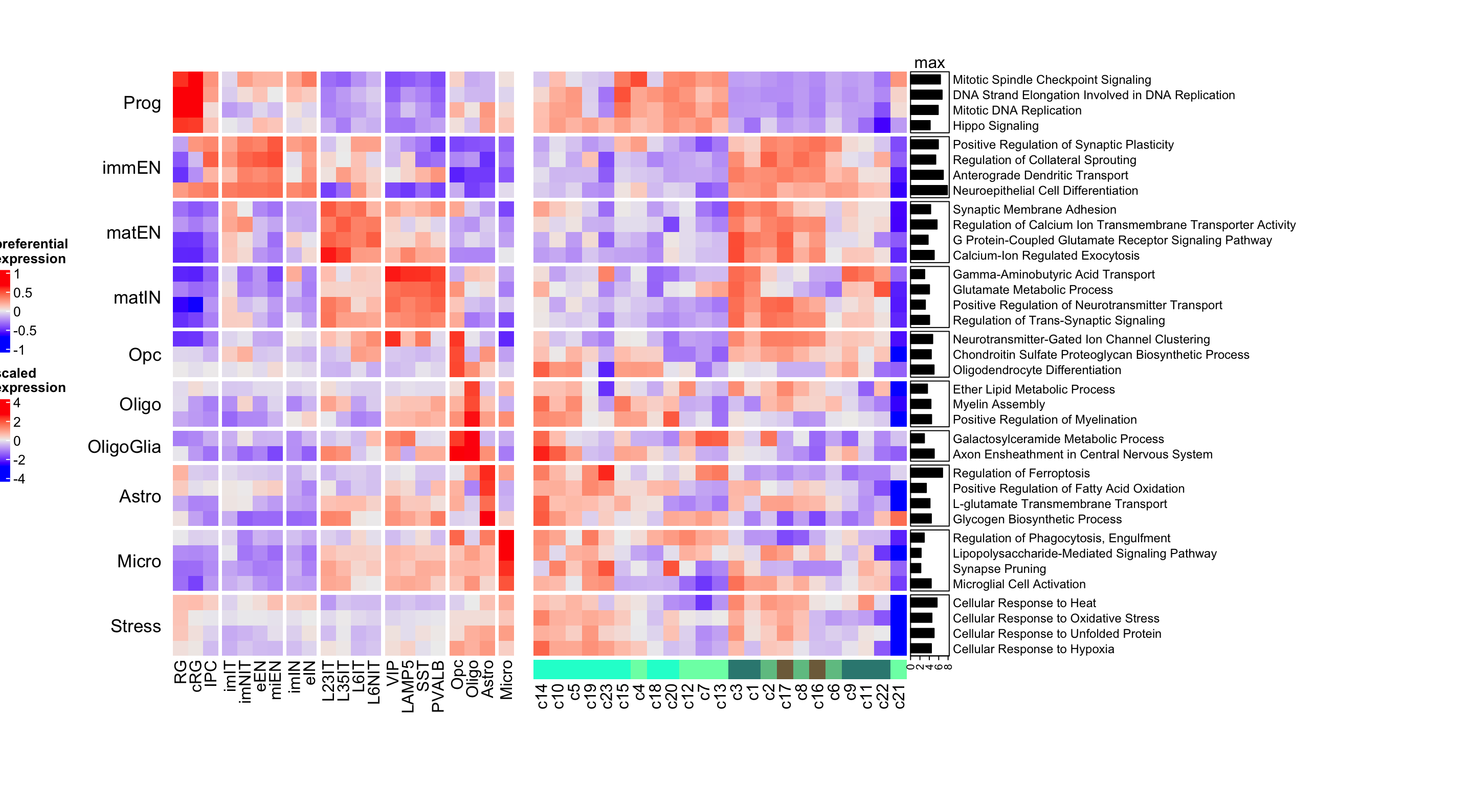
Figure 5.7: Heatmap of corticogenesis-specific GO biological processes in resource and mapped clusters.
This heatmap shows that the biological processes match the annotations, with radial glia clusters displaying higher expression of processes associated with proliferation and glial metabolism, but we can also see that clusters 19 and 23 show high expression of stress-related processes, while displaying low expression of the terms more related to radial glia, their assigned annotation. This could explain why cluster 23 has such a low mapping confidence and suggests that these clusters are composed by possibly stressed cells.
The same type of analysis can be done with the neurogenesis network:Show the code (neurogenesis GO code)
sc_seu_neuro_GOBP <- do.call(rbind, lapply(neurogenesis_GO, function(g) {

  g <- g[which(g %in% rownames(sc_seu))]

  Matrix::colMeans(logcounts(sc_pseudo)[g,])

}))

rownames(sc_seu_neuro_GOBP) <- gsub(" \\(GO:[0-9]+\\)$", "", rownames(sc_seu_neuro_GOBP))
sc_seu_neuro_GOBP <- sc_seu_neuro_GOBP[,mixedorder(colnames(sc_seu_neuro_GOBP))]


neuro_gobp_pe <- neurogenesis_preferential_GO$GO_Biological_Process_2025$activity[names(neurogenesis_GO),]


neuroTrends <- do.call(cbind, lapply(rownames(neuro_gobp_pe), function(i)
  smooth.spline(1:length(neuro_gobp_pe[i,]),
                neuro_gobp_pe[i,], spar = 1)$y))

colnames(neuroTrends) <- rownames(neuro_gobp_pe)

neuroTrends <- t(neuroTrends)[names(neurogenesis_GO),]
neuroTrends <- neuroTrends[order(apply(neuroTrends, 1, which.max), Matrix::rowMeans(neuroTrends)),]

rownames(neuroTrends) <- gsub(" \\(GO:[0-9]+\\)$", "", rownames(neuroTrends))

stage_palette <- unique(neurogenesis_sce$Stages_color)
names(stage_palette) <- unique(neurogenesis_sce$Stages)

h1 <- Heatmap(t(scale(t(neuroTrends))),
              cluster_columns = F,
              cluster_rows = F,
              bottom_annotation = HeatmapAnnotation(df=data.frame(stage=neurogenesis_sce$Stages),
                                                    col=list(stage=stage_palette),
                                                    show_legend = F,
                                                    show_annotation_name = F),
              name = 'inferred expression\n(z scaled)',
              height = unit(100, 'mm'),
              width = unit(30, 'mm'))

ht2 <- Heatmap(
  t(scale(t(sc_seu_neuro_GOBP[rownames(neuroTrends),]))),
  name = 'scaled\nexpression',
  width = unit(ncol(sc_seu_neuro_GOBP) * 4.2, 'mm'),
  cluster_columns = TRUE,
  row_names_gp = gpar(fontsize = 9,
                      fontface =ifelse(colnames(t(scale(t(sc_seu_neuro_GOBP[rownames(neuroTrends),])))) %in% c("c23"), "bold", "plain")),
  right_annotation = rowAnnotation(max = anno_barplot(apply(sc_seu_neuro_GOBP[rownames(neuroTrends),], 1, max),
                                                      gp = gpar(fill = 'black')),
                                   annotation_name_side = 'top',
                                   annotation_name_rot = 0),
  bottom_annotation = HeatmapAnnotation(annotation = mapped_sc_pseudo$annotation$Best.Annotation[colnames(sc_seu_cortico_GOBP)],
                                        col = list(annotation = corticogenesis_palette),
                                        show_legend = FALSE,
                                        show_annotation_name = FALSE),
  show_column_dend = FALSE
)


ht_list <- h1 + ht2

draw(ht_list, heatmap_legend_side = "left")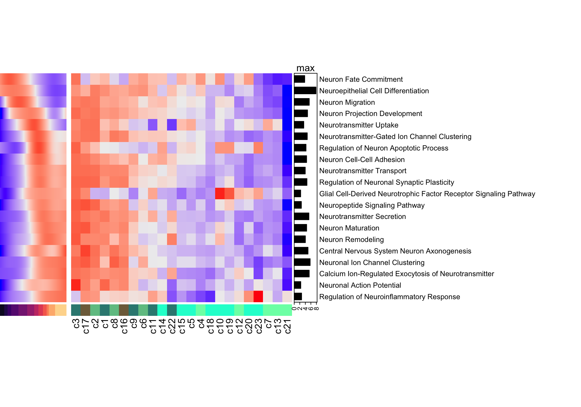
Figure 5.8: Heatmap of neurogenesis-specific GO biological processes in resource and mapped clusters.
Again, the cluster with the highest neuroinflammatory response (indicative of stress) is cluster 23. Thanks to the use of the neurogenesis-specific network we can appreciate how neuronal specific processes are expressed in clusters assigned to the immature neuron annotations and not in those labelled as progenitors.
Additionally, we can visualize the mapped points directly on the eTraces, to see how similar they are to clusters in the resource network based on gene expression. The function to perform such analysis is map_eTrace, which requires the following inputs:
-
net= the reference network to use. -
mapped_obj= the result of mapNetwork. - the inputs required to run plot_eTrace (see the Chapter Analysis tools), mainly
genes,expression_enrichment, andclusters_comparison.
map_eTrace(net = corticogenesis_sce,
         mapped_obj = mapped_sc_pseudo,
         genes = "VIM",
         main = "VIM",
         expression_enrichment = TRUE,
         clusters_comparison = TRUE)

map_eTrace(net = corticogenesis_sce,
         mapped_obj = mapped_sc_pseudo,
         genes = "SYT1",
         main = "SYT1",
         expression_enrichment = TRUE,
         clusters_comparison = TRUE)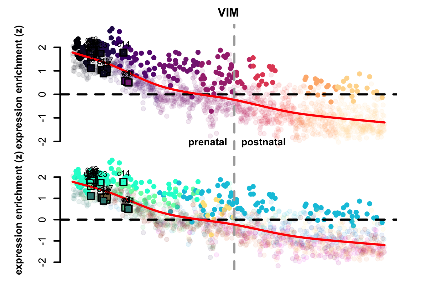
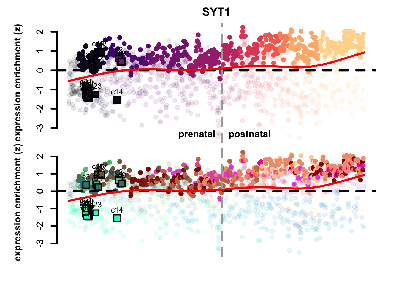
Figure 5.9: VIM and SYT1 eTrace in corticogenesis and mapped points
From this type of analysis we can clearly appreciate the distinction between radial glia-like clusters and more neuronal ones. Additionally, we can see at a glance which mapped points resemble more mature reference clusters, as age increases from left to right. The more rightward clusters are: 2, 9, 11, and 14. If we check the percentage of cells belonging to the latest time point (4 months) across each cluster, we can see that those clusters are also those with the highest proportion of latest-stage cells:
sort(apply(table(sc_seu$stage, paste0('c', sc_seu$seurat_clusters)), 2, function(i) {i/sum(i)})['Organoid-4M',]*100)
#>        c12        c13        c17        c20        c21
#>  0.0000000  0.0000000  0.0000000  0.0000000  0.0000000
#>        c22         c7        c16        c18        c10
#>  0.0000000  0.0000000  0.2590674  0.2857143  0.8968610
#>         c8         c3         c6         c5        c15
#>  1.2219959  1.3736264  3.2374101  4.3478261  8.7281796
#>        c19         c4         c1        c23         c2
#>  9.7826087 10.3395062 11.1006585 11.7647059 42.8571429
#>        c14        c11         c9
#> 44.0097800 47.1655329 53.0303030
We can also obtain markers for each cluster using the Seurat function FindAllMarkers and plot those genes in the eTraces.
markers <- FindAllMarkers(sc_seu,
                          only.pos = TRUE,
                          min.pct = 0.5,
                          logfc.threshold = 1)

markers <- markers[which(markers$p_val_adj < 0.001),]

markers <- split(markers$gene, markers$cluster)
lapply(names(markers), function(i) {
        g <- markers[[i]]
        g <- g[which(g %in% rownames(corticogenesis_sce))]
        plot_eTrace(net = corticogenesis_sce,
                    genes = g,
                    main = paste("markers of cluster",i))
})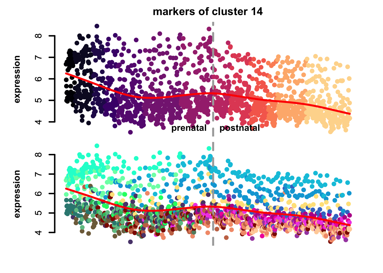
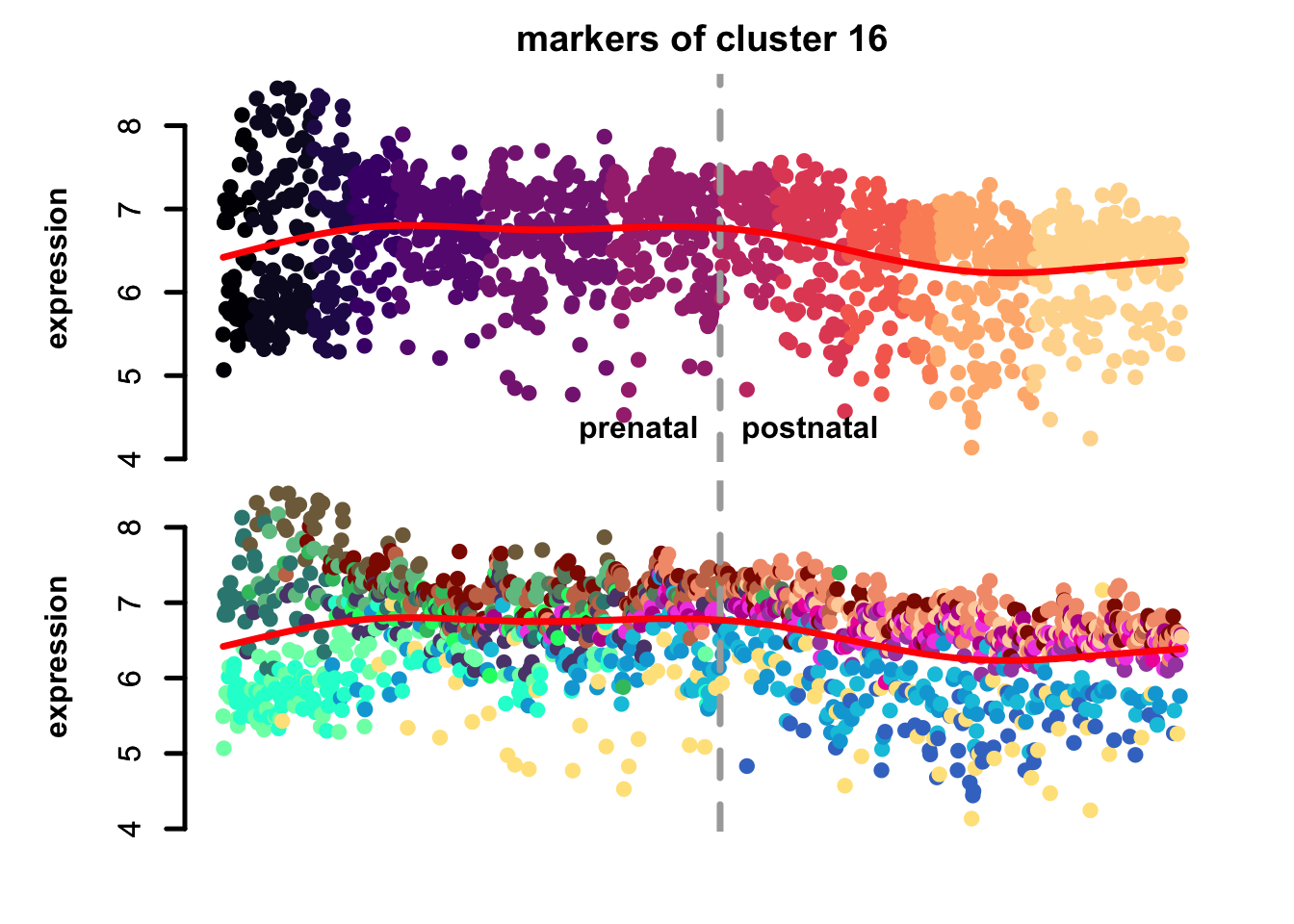
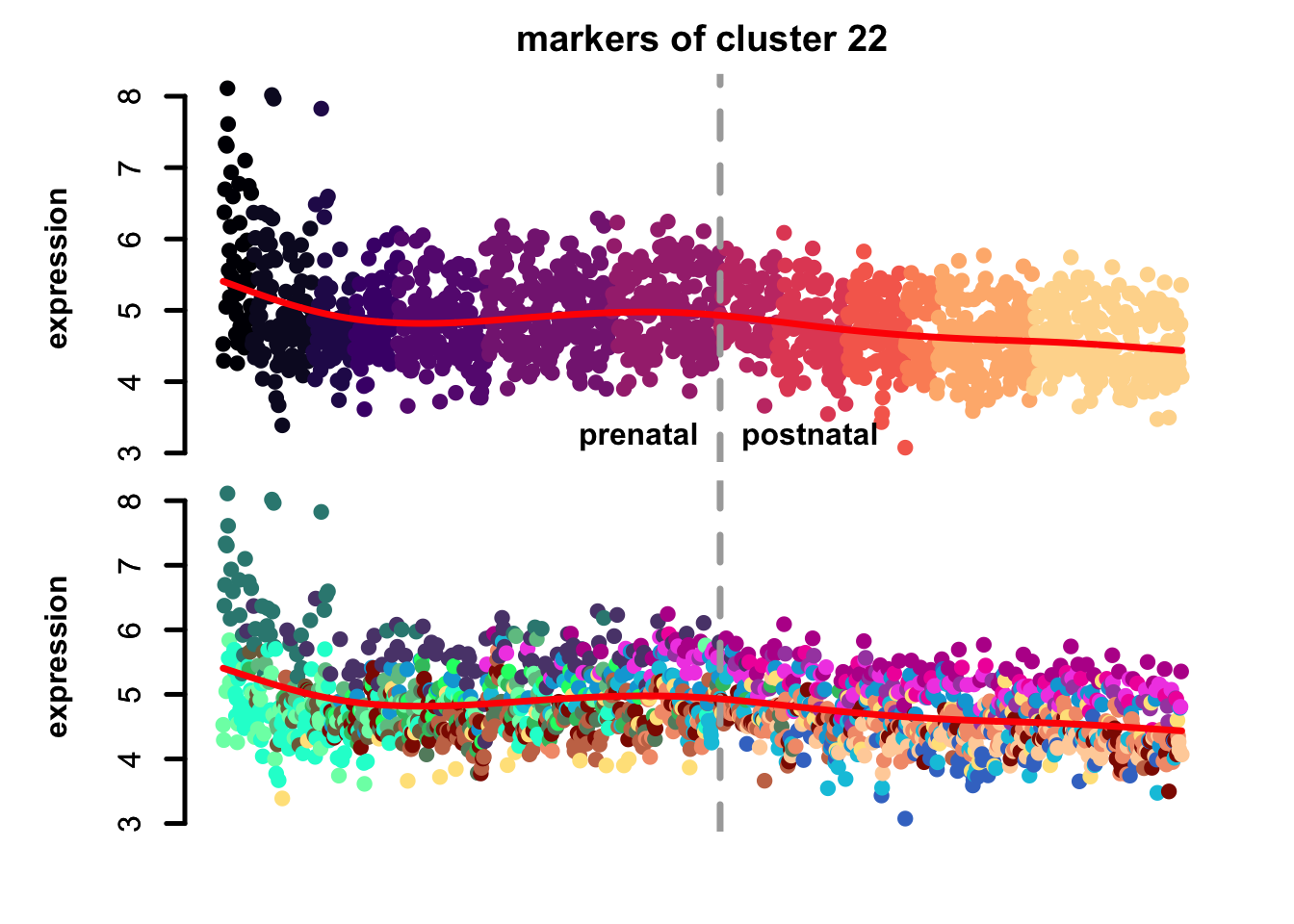
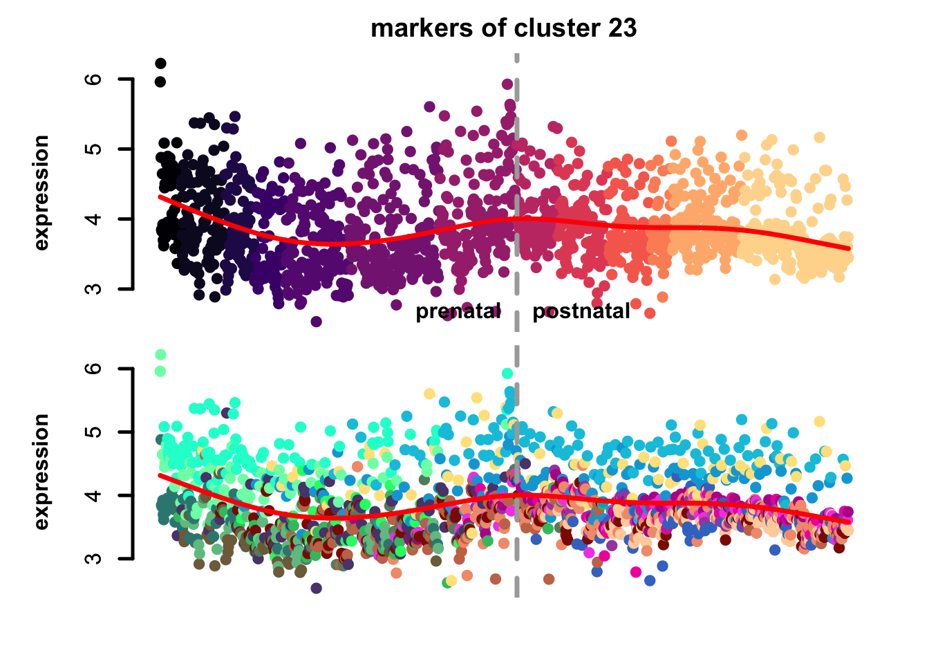
Figure 5.10: eTraces of markers of selected clusters.
Again, it is easy to distinguish between more neuronal clusters and more radial glia-like clusters, but also we can find some clusters that are more inhibitory neurons-like (e.g. clusters 22 and 11), and cluster 23 markers which are highly expressed in microglia too, again pointing to a possible stress-related transcriptional signature.