3 Analysis Tools

3.1 Loading necessary libraries and data

3.1.1 Loading the right libraries

# functions package
library(neuRoDev)
# extra packages
library(ComplexHeatmap)

3.1.2 Loading the networks necessary objects

corticogenesis_sce <- corticogenesis.sce(directory = '~/Downloads')
neurogenesis_sce <- neurogenesis.sce(directory = '~/Downloads')
gliogenesis_sce <- gliogenesis.sce(directory = '~/Downloads')

3.2 eTraces

We developed an intuitive way to directly visualize a molecular phenotype score in each cluster of our reference networks, which we called eTrace (expression Trace). We provide here an interactive tool to directly assess the (log-normalized) expression of input genes and gene sets, as well as the expression enrichment trends (more statistically robust).

The function used to visualize eTraces is plot_eTrace. The function requires few inputs, with the only mandatory one being the reference network (net):

net= the reference network to use.
genes= a specific gene or set of genes from which to derive the score to plot. If more genes are given, the output will be an averaged score of those genes. It defaults to NULL, as the user can directly provide a score per cluster (see score). If no genes are given and a score matrix is selected, all genes in the score matrix will be considered.
score= it can be a vector, with one value per cluster, or a matrix. If a matrix is given together with genes (see genes), only the values of the selected genes that are present in the matrix will be shown. It defaults to the log-normalized expression values contained in net under logcounts.
expression_enrichment= it defines whether to compute expression enrichment of the given genes, a more statistically robust way of looking at the expression. If TRUE, the score that will be used will be the expression enrichment score, regardless on what is put in score. It defaults to FALSE.
add_sig_line= it defines whether to add horizontal lines to define the boundaries between statistically significant or not. It defaults to TRUE and works only if expression_enrichment is also set to TRUE. The p-value for which the lines are drawn is defined by pval_threshold. Here the statistical significance is derived comparing the expression of the genes with the expression of randomly selected genes for each cluster.
clusters_comparison= it defines whether to highlight clusters that have a statistically higher expression compared to other clusters. It defaults to FALSE and works only if expression_enrichment is set to TRUE. The p-value for which the clusters are highlighted is defined by pval_threshold. Here the statistical significance is derived comparing the expression of the genes across clusters, not with other genes.
other plotting and fine-tuning inputs, see ?plot_eTrace for further information.

plot_eTrace(corticogenesis_sce, 
            genes = 'SST', 
            main = 'SST - no enrichment')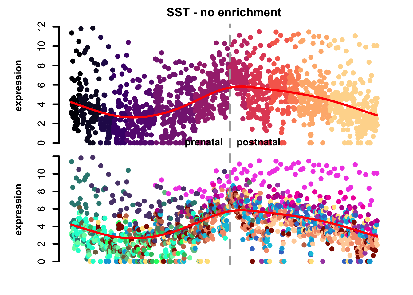

Figure 3.1: Single gene eTrace in corticogenesis.

plot_eTrace(corticogenesis_sce, 
            genes = 'GFAP', 
            expression_enrichment = TRUE, 
            main = 'GFAP - enrichment', 
            add_sig_line = TRUE)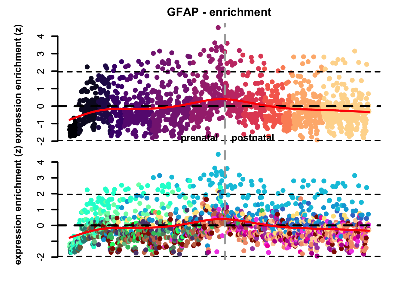

Figure 3.2: Single gene expression enrichment eTrace in corticogenesis.

plot_eTrace(corticogenesis_sce, 
            genes = 'PAX6', 
            expression_enrichment = TRUE, 
            main = 'PAX6 - enrichment', 
            clusters_comparison = TRUE)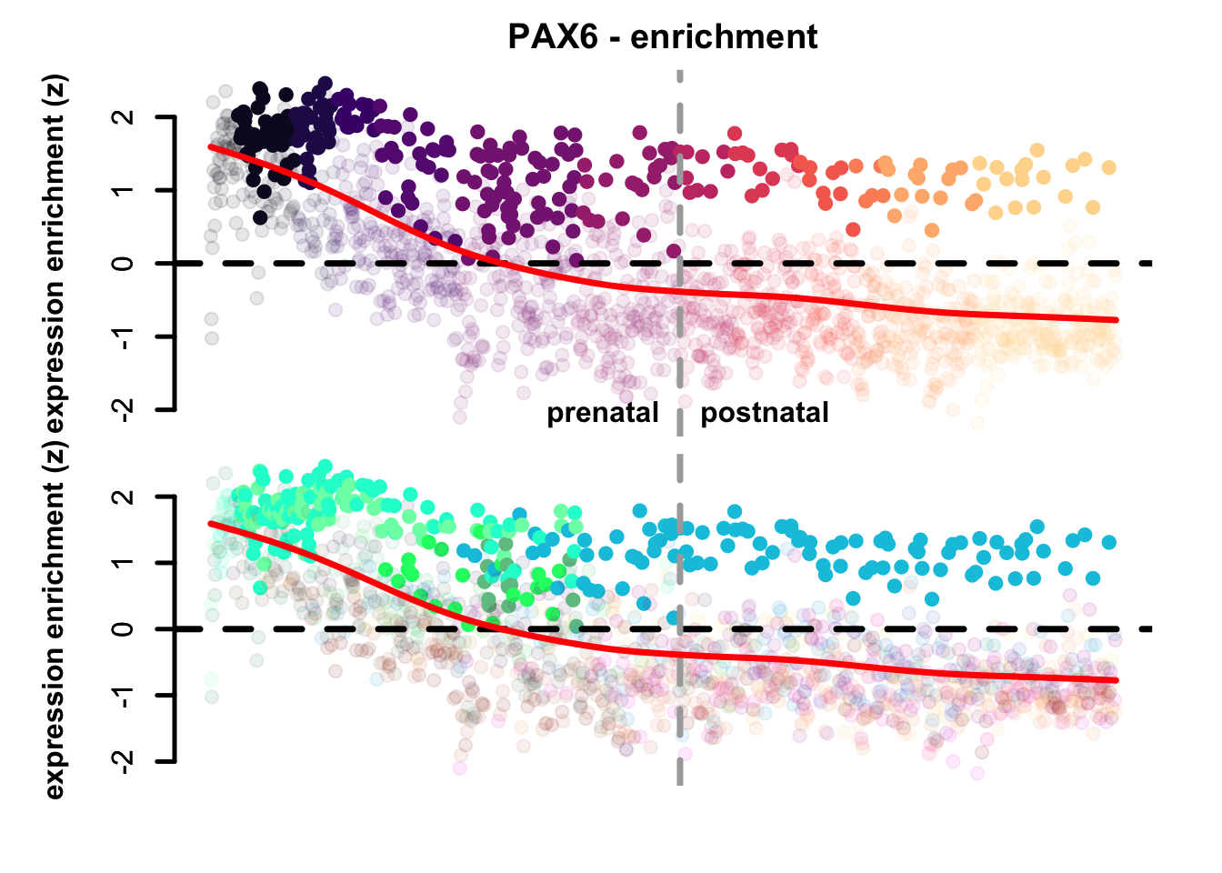

Figure 3.3: Single gene expression enrichment eTrace and statistical highlight in corticogenesis.

It is possible to inspect not only single genes but also gene sets. For example, we can visualize the expression of curated preferentially expressed genes in the reference subclasses. The objects are available for download here (PreferentialExpression folder).

corticogenesis_pe_genes <- readRDS("~/Downloads/corticogenesis_subclass_preferential_genes.rds")
neurogenesis_pe_genes <- readRDS("~/Downloads/neurogenesis_subclass_preferential_genes.rds")
gliogenesis_pe_genes <- readRDS("~/Downloads/gliogenesis_subclass_preferential_genes.rds")

plot_eTrace(corticogenesis_sce, 
            genes = corticogenesis_pe_genes$Oligo, 
            main = 'Oligodendrocyte preferentially expressed genes')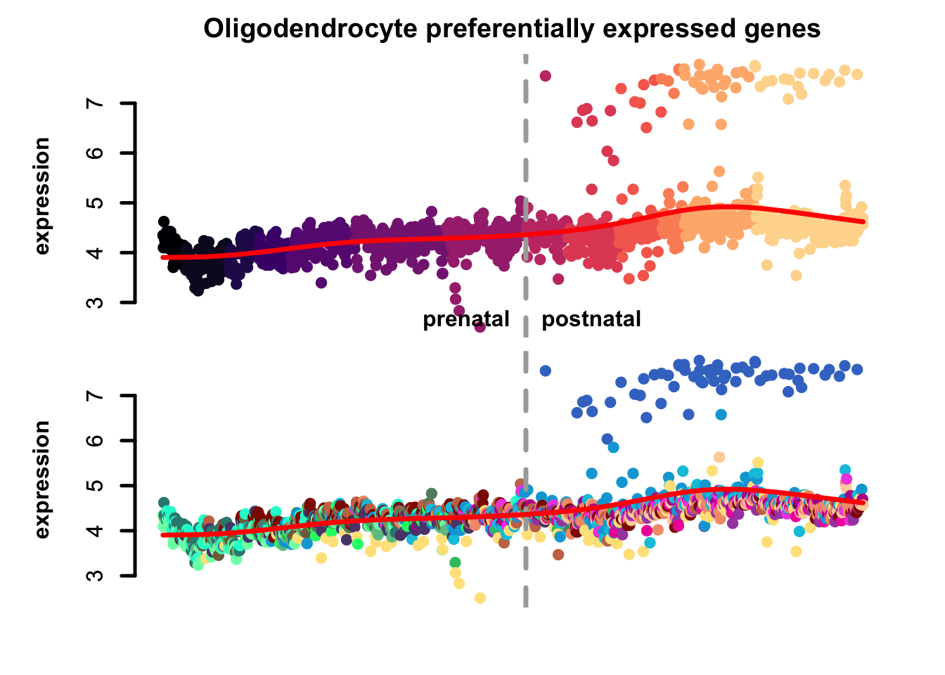

Figure 3.4: Gene set eTrace in corticogenesis.

plot_eTrace(corticogenesis_sce, 
            genes = corticogenesis_pe_genes$Opc, 
            expression_enrichment = TRUE, 
            main = 'OPC preferentially expressed genes', 
            add_sig_line = TRUE)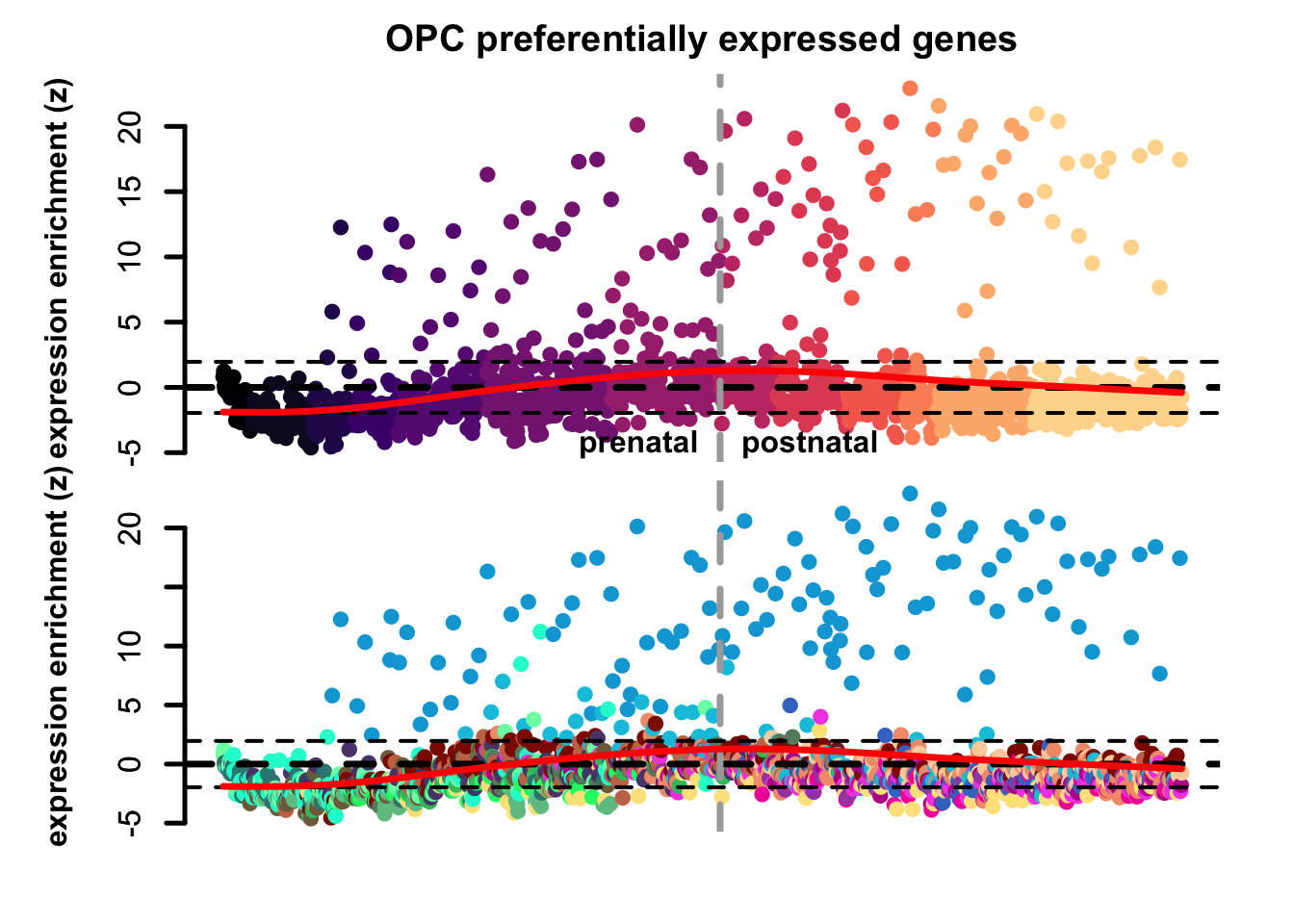

Figure 3.5: Genes set expression enrichment eTrace in corticogenesis.

Any kind of score can be visualized with the eTrace. As a further example, we can visualize the preferential expression of Gene Ontology genesets.

We have already computed preferential expression of Gene Ontology Biological Processes (BP), Molecular Functions (MF), and Cellular Components (CC), which can be downloaded here (PreferentialExpression folder). Each object is a list containing preferential expression scores in one of the three reference networks in the three ontologies (BP, MF, CC). Each element of each list contains the activity (activity) derived from Gene Set Variation Analysis (one value per gene set in each cluster) and the preferential expression scores (preferential; one value per gene set in each subclass).

corticogenesis_preferential_GO <- readRDS('~/Downloads/corticogenesis_preferential_GO.rds')
neurogenesis_preferential_GO <- readRDS('~/Downloads/neurogenesis_preferential_GO.rds')
gliogenesis_preferential_GO <- readRDS('~/Downloads/gliogenesis_preferential_GO.rds')

plot_eTrace(corticogenesis_sce, 
            score = corticogenesis_preferential_GO$GO_Biological_Process_2025$activity["Glycogen Biosynthetic Process (GO:0005978)",], 
            main = 'Glycogen Biosynthesis')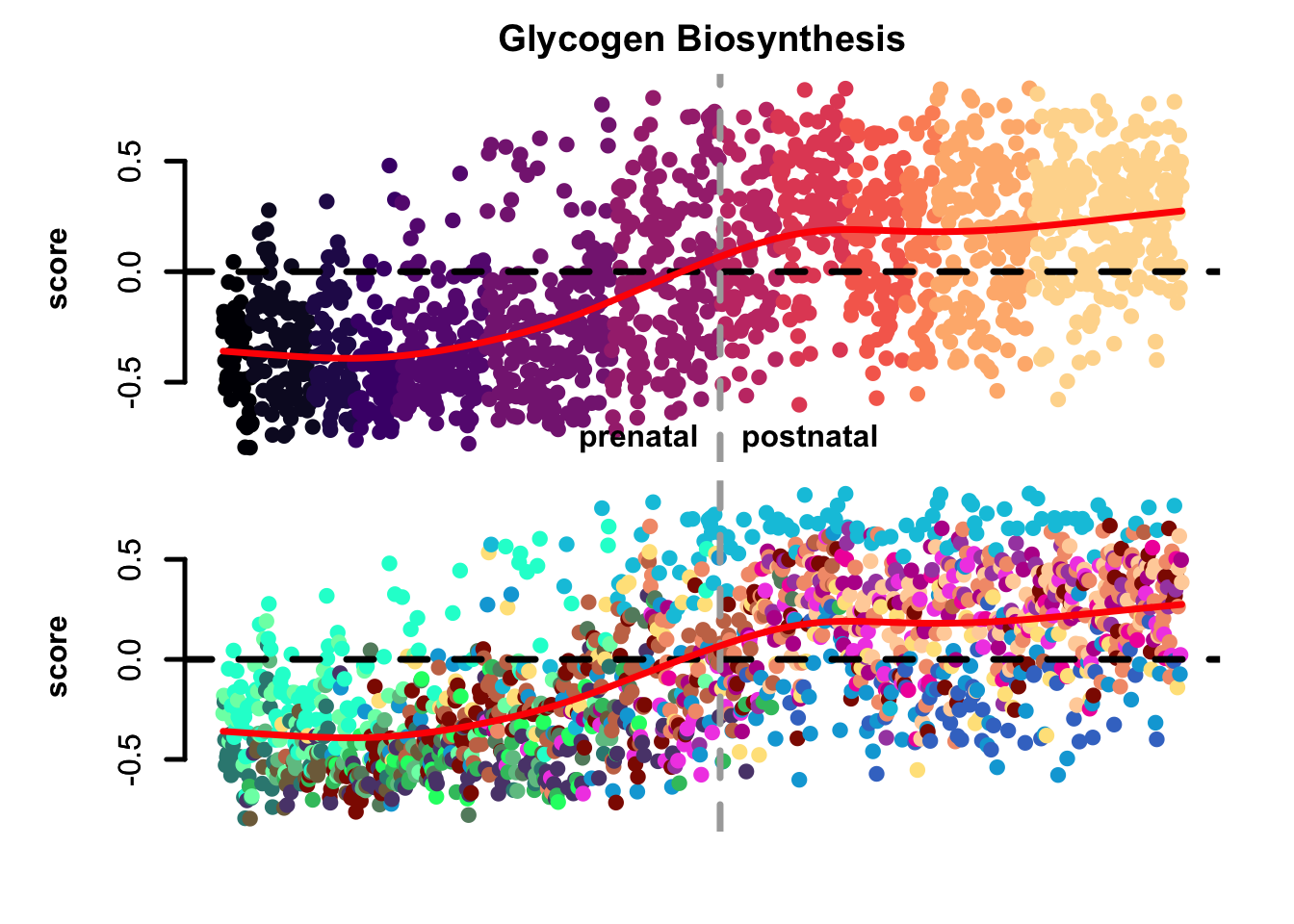

Figure 3.6: Gene set activity score eTrace in corticogenesis.

The expression enrichment values can be obtained by using the function get_eTrace, which requires as input: - net= the reference network. - genes= the genes to use.

Additionally, it is possible to look at within-lineage specific patterns of expression by subsetting the networks. For example, here we show the expression patterns of genes inside the astrogenesis- and oligodendrogenesis-specific trajectories of differentiation:

astro_sce <- gliogenesis_sce[,-c(grep(gliogenesis_sce$SubClass, pattern="OPC"),
  grep(gliogenesis_sce$SubClass, pattern="Oli"))] #removes everything that is oligodendroglia-related

oli_sce <- gliogenesis_sce[,c(grep(gliogenesis_sce$SubClass, pattern="OPC"),
  grep(gliogenesis_sce$SubClass, pattern="Oli"))] #keeps only oligodendroglia-related
oli_sce <- oli_sce[,order(oli_sce$Days)]

plot_eTrace(astro_sce,
            genes = "SPARCL1",
            expression_enrichment = TRUE,
            main = "SPARCL1 in astrogenesis")

plot_eTrace(oli_sce,
            genes = "MAG",
            expression_enrichment = TRUE,
            main = "MAG in oligodendrogenesis",
            clusters_comparison = TRUE)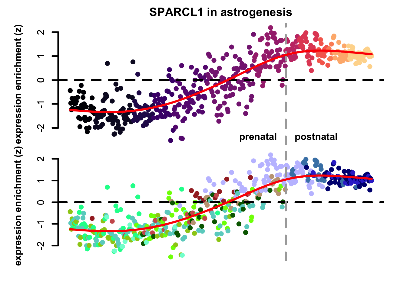

Figure 3.7: Single gene expression enrichment eTrace within astrogenesis.

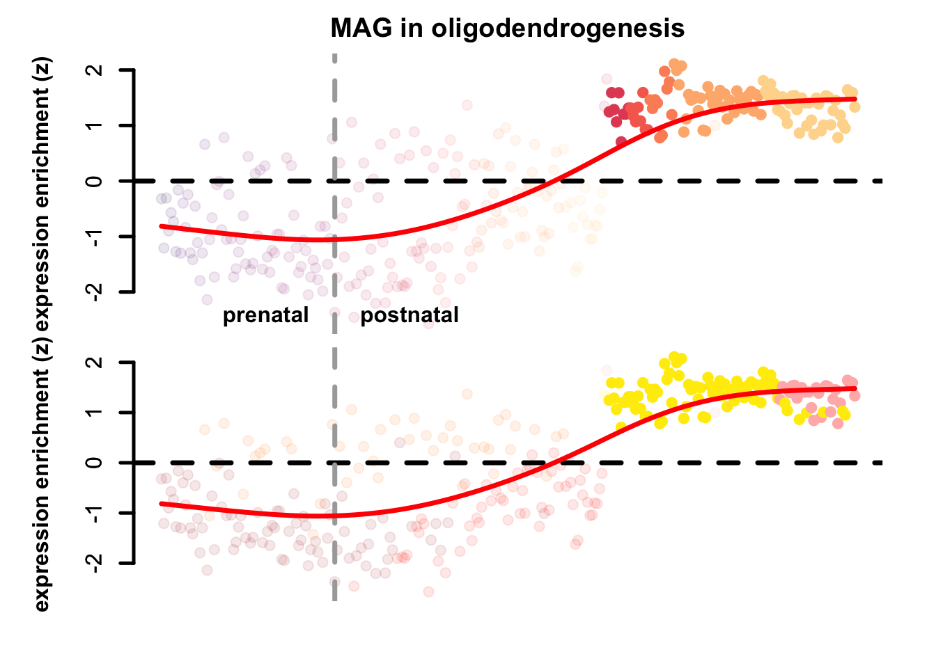
Figure 3.8: Single gene expression enrichment eTrace within oligodendrogenesis.

To obtain the results and details of the statistical analysis performed by setting clusters_comparison to TRUE, you can directly use the compare_clusters function, that uses as input the network (net) and the tested gene(s) (genes). Additionally, you can specify if you want to test the expression enrichment differences (default) or the base expression (expression_enrichment = FALSE). You can also set the statistical significance threshold with pval_threshold.

Here is an example:

gfap_comparison <- compare_clusters(net = corticogenesis_sce, genes = 'GFAP')

Under GlobalTest you have the summary of the result of a linear model that assesses if the gene expression/enrichment in each subclass-stage group is statistically higher than 0. Here we will show only the first few lines:

head(gfap_comparison$GlobalTest)
#>                    Estimate Std. Error    t value
#> cRG.1-embryonic   -1.243599  0.1810367  -6.869319
#> RG.1-embryonic    -1.283313  0.1349368  -9.510474
#> imNIT.1-embryonic -1.580875  0.5724884  -2.761410
#> eEN.1-embryonic   -1.298802  0.5724884  -2.268696
#> eIN.1-embryonic   -1.490208  0.1388488 -10.732589
#> imIN.1-embryonic  -1.034597  0.5724884  -1.807193
#>                       Pr(>|t|)
#> cRG.1-embryonic   9.634398e-12
#> RG.1-embryonic    7.832039e-21
#> imNIT.1-embryonic 5.829627e-03
#> eEN.1-embryonic   2.343689e-02
#> eIN.1-embryonic   6.880401e-26
#> imIN.1-embryonic  7.094444e-02

Under ByStageTests you have the results of the Wilcoxon tests done for each stage independently, comparing each subclass in that stage to all the other subclasses in that stage. Here we will print only the comparisons in the first stage:

gfap_comparison$ByStageTests[[1]]
#> $`RG.2A-early_prenatal`
#> 
#>  Wilcoxon rank sum test with continuity correction
#> 
#> data:  score[which(sub_net$SubClass == subclass)] and score[which(sub_net$SubClass != subclass)]
#> W = 1712, p-value = 2.041e-06
#> alternative hypothesis: true location shift is greater than 0
#> 
#> 
#> $`cRG.2A-early_prenatal`
#> 
#>  Wilcoxon rank sum test with continuity correction
#> 
#> data:  score[which(sub_net$SubClass == subclass)] and score[which(sub_net$SubClass != subclass)]
#> W = 760, p-value = 0.3101
#> alternative hypothesis: true location shift is greater than 0
#> 
#> 
#> $`Micro.2A-early_prenatal`
#> 
#>  Wilcoxon rank sum test with continuity correction
#> 
#> data:  score[which(sub_net$SubClass == subclass)] and score[which(sub_net$SubClass != subclass)]
#> W = 111, p-value = 0.3791
#> alternative hypothesis: true location shift is greater than 0

3.3 Interactive eTrace

To explore the normalized expression and expression enrichment levels of (single) genes it is possible to use this interactive tool and observe in a glance patterns over ~70 years of life. Below you can access with one click to the three different resources and give as input a single gene or a gene set and look at the patterns of expression in time and through subclasses.

🔍 Click here to interactively visualize the corticogenesis eTrace

🔍 Click here to interactively visualize the neurogenesis eTrace

🔍 Click here to interactively visualize the gliogenesis eTrace

3.4 Expression enrichment across stage and subclass

An alternative and compact visualization of expression enrichment in both subclasses and stages can be obtained by using the function plot_eMatrix. The inputs are listed below, and are the same as those needed by the get_eTrace function:

net= the reference network to use.
genes= a specific gene or set of genes from which to derive the expression enrichment.
nRand= the number of random sets to use for the expression enrichment calculation. Defaults to 100.
mask= defines if setting all values not statistically significant to 0. The statistical significance threshold is defined by pval_threshold.

This returns an eMatrix showing on the columns subclasses, on the rows stages, and the values represent enrichment scores.

Show the code (plotting eMatrix)

plot_eMatrix(net = neurogenesis_sce, 
             genes = 'NEUROD6')
plot_eMatrix(net = gliogenesis_sce, 
             genes = 'GFAP')
plot_eMatrix(net = corticogenesis_sce, 
             genes = corticogenesis_pe_genes$L6NIT)

plot_eMatrix(net = corticogenesis_sce, 
             genes = 'VIP')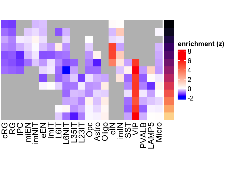

Figure 3.9: VIP eMatrix in corticogenesis.

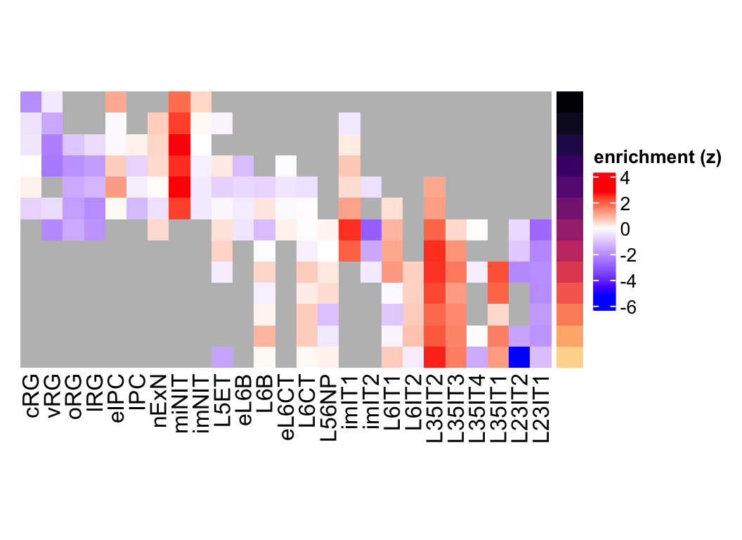
Figure 3.10: NEUROD6 eMatrix in neurogenesis.

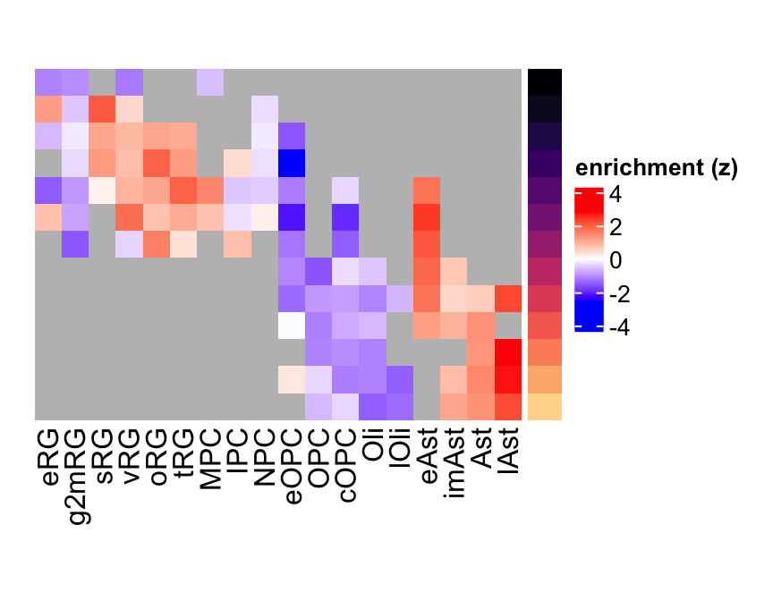
Figure 3.11: GFAP eMatrix in gliogenesis.

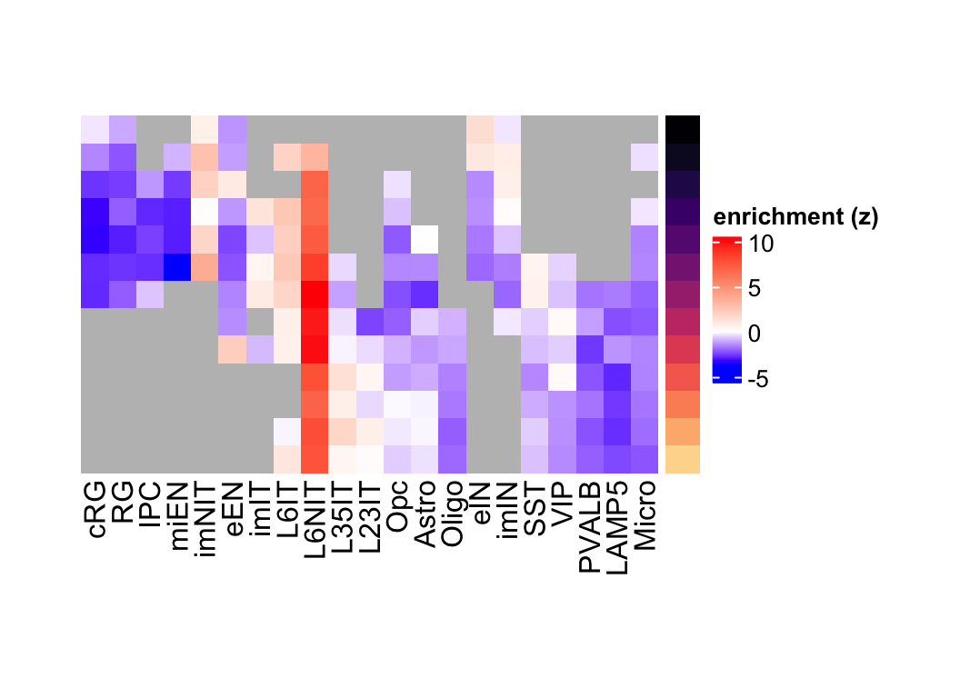
Figure 3.12: L6NIT preferentially expressed genes eMatrix in corticogenesis.

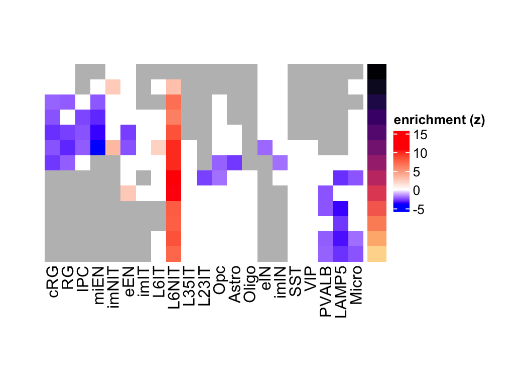
Figure 3.13: L6NIT preferentially expressed genes eMatrix in corticogenesis highlighting statistical significance.

It is possible to obtain the eMatrix itself by using the function get_eMatrix, which uses the same inputs as plot_eMatrix.

3.5 Visualization of enrichment in the network

As described in Chapter Network exploration, we can visualize cluster-wise scores directly in the UMAP at the network level. This can be done with the plotNetworkScore function, setting expression_enrichment to TRUE.

plotNetworkScore(net = corticogenesis_sce, 
                 genes = corticogenesis_pe_genes$Oligo, 
                 expression_enrichment = TRUE,
                 main = "Enrichment: Oligo preferential genes")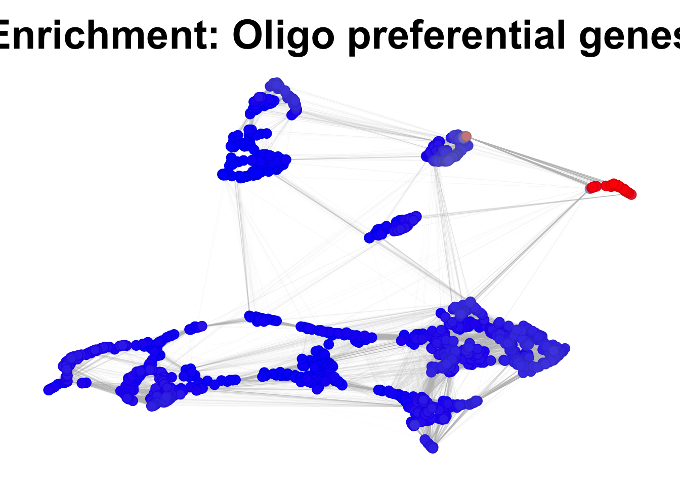

Figure 3.14: Gene expression enrichment in the corticogenesis network.

3.6 Preferential expression

The reference networks also contain the pseudobulks of each subclass and each stage, along with the preferential expression profiles computed between subclasses/stages. We can inspect the genes with the highest preferential expression scores in each subclass.

Show the code (plotting heatmaps)

top_genes_cortico <- unique(rownames(corticogenesis_sce)[apply(assays(corticogenesis_sce@metadata$subclass_psb)[['preferential']], 2, function(i) {
  order(i, decreasing =  TRUE)[1:5]})])

h_cortico <- Heatmap(t(assays(corticogenesis_sce@metadata$subclass_psb)[['preferential']][top_genes_cortico, levels(corticogenesis_sce$SubClass)]), 
  name = 'preferential\nexpression', 
  cluster_columns = TRUE,
  cluster_rows = FALSE,
  height = grid::unit(ncol(assays(corticogenesis_sce@metadata$subclass_psb)[['preferential']])*4, 'mm'), 
  width = grid::unit(length(top_genes_cortico)*4, 'mm'),
  rect_gp = gpar(color = 'black', lwd = 0.5))

draw(h_cortico, , heatmap_legend_side = 'left')

top_genes_neuro <- unique(rownames(neurogenesis_sce)[apply(assays(neurogenesis_sce@metadata$subclass_psb)[['preferential']], 2, function(i) {
  order(i, decreasing =  TRUE)[1:5]})])

h_neuro <- Heatmap(t(assays(neurogenesis_sce@metadata$subclass_psb)[['preferential']][top_genes_neuro, levels(neurogenesis_sce$SubClass)]), 
  name = 'preferential expression', 
  cluster_columns = TRUE,
  cluster_rows = FALSE,
  height = grid::unit(ncol(assays(neurogenesis_sce@metadata$subclass_psb)[['preferential']])*4, 'mm'), 
  width = grid::unit(length(top_genes_neuro)*4, 'mm'), 
  rect_gp = gpar(color = 'black', lwd = 0.5))

draw(h_neuro, , heatmap_legend_side = 'left')

top_genes_glio <- unique(rownames(gliogenesis_sce)[apply(assays(gliogenesis_sce@metadata$subclass_psb)[['preferential']], 2, function(i) {
  order(i, decreasing =  TRUE)[1:5]})])

h_glio <- Heatmap(t(assays(gliogenesis_sce@metadata$subclass_psb)[['preferential']][top_genes_glio, levels(gliogenesis_sce$SubClass)]), 
  name = 'preferential expression', 
  cluster_columns = TRUE,
  cluster_rows = FALSE,
  height = grid::unit(ncol(assays(gliogenesis_sce@metadata$subclass_psb)[['preferential']])*4, 'mm'),
  width = grid::unit(length(top_genes_glio)*4, 'mm'), 
  rect_gp = gpar(color = 'black', lwd = 0.5))

draw(h_glio, , heatmap_legend_side = 'left')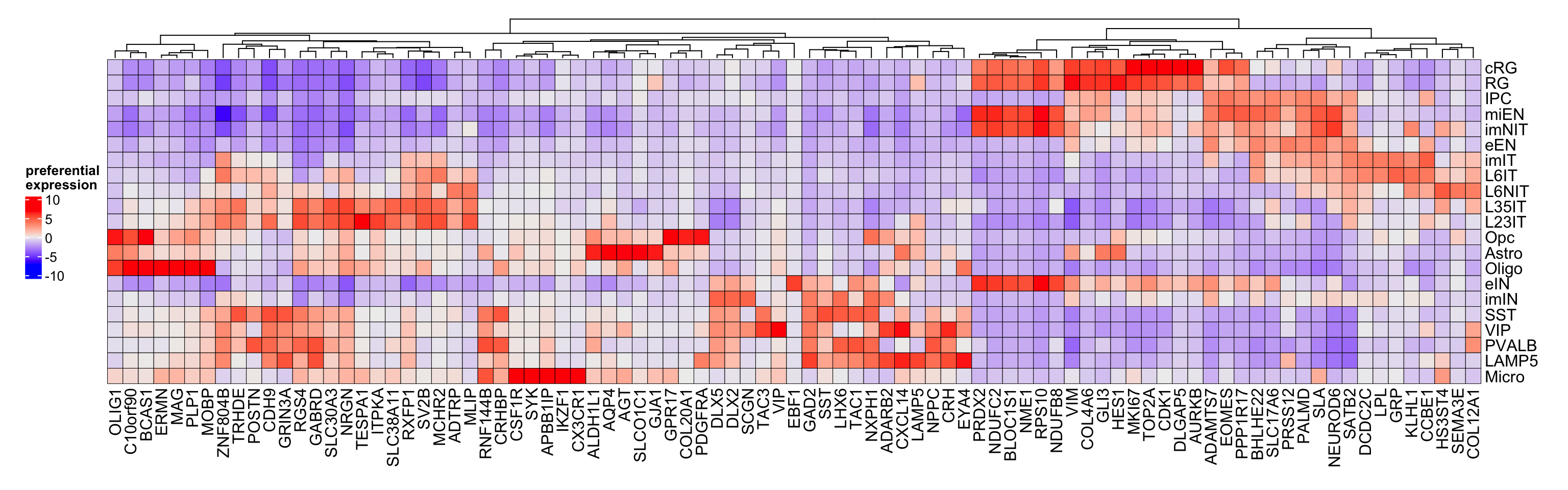

Figure 3.15: Top preferential genes in corticogenesis.

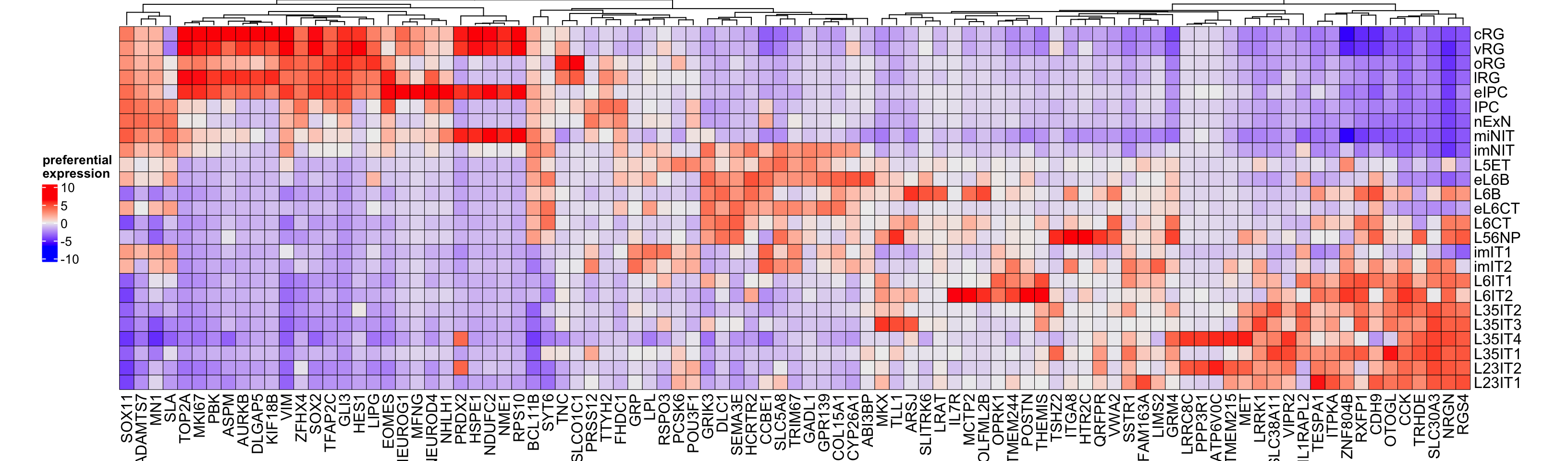
Figure 3.16: Top preferential genes in neurogenesis.

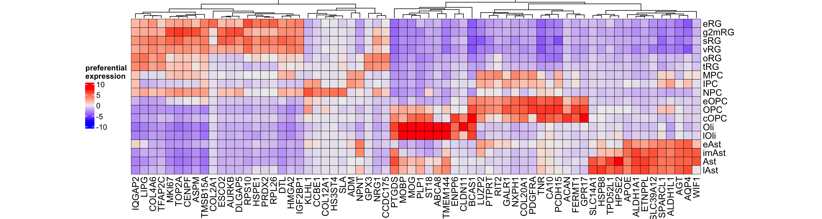
Figure 3.17: Top preferential genes in gliogenesis.

At the same time, we computed the preferential expression scores for Gene Ontology gene sets. As an example, we can visualize the preferential expression scores of Gene Ontology Biological Processes.

Show the code (plotting heatmaps)

top_GO_bp_cortico_list <- apply(corticogenesis_preferential_GO$GO_Biological_Process_2025$preferential, 2, function(i) {
  rownames(corticogenesis_preferential_GO$GO_Biological_Process_2025$preferential)[order(i, decreasing = TRUE)[seq(1,2)]]
  }
) #selecting top 2 processes by subclass

top_GO_bp_cortico <- corticogenesis_preferential_GO$GO_Biological_Process_2025$preferential[unique(as.vector(top_GO_bp_cortico_list)),]

rownames(top_GO_bp_cortico) <- sub("\\s*\\(GO:\\d+\\)$", "", rownames(top_GO_bp_cortico))

h <- Heatmap(top_GO_bp_cortico[,levels(corticogenesis_sce$SubClass)], 
             name = 'preferential\nexpression', 
             width = grid::unit(ncol(top_GO_bp_cortico)*4, 'mm'), 
             height = grid::unit(nrow(top_GO_bp_cortico)*4, 'mm'), 
             cluster_columns = FALSE, 
             rect_gp = gpar(color = 'black', lwd = 0.5))
draw(h, heatmap_legend_side = 'left')

top_GO_bp_neuro_list <- apply(neurogenesis_preferential_GO$GO_Biological_Process_2025$preferential, 2, function(i) {
  rownames(neurogenesis_preferential_GO$GO_Biological_Process_2025$preferential)[order(i, decreasing = TRUE)[seq(1,2)]]
  }
)

top_GO_bp_neuro <- neurogenesis_preferential_GO$GO_Biological_Process_2025$preferential[unique(as.vector(top_GO_bp_neuro_list)),]

rownames(top_GO_bp_neuro) <- sub("\\s*\\(GO:\\d+\\)$", "", rownames(top_GO_bp_neuro))

h_neuro <- Heatmap(top_GO_bp_neuro[,levels(neurogenesis_sce$SubClass)], 
                   name = 'preferential\nexpression', 
                   width = grid::unit(ncol(top_GO_bp_neuro)*4, 'mm'), 
                   height = grid::unit(nrow(top_GO_bp_neuro)*4, 'mm'), 
                   cluster_columns = FALSE, 
                   rect_gp = gpar(color = 'black', lwd = 0.5))
draw(h_neuro, heatmap_legend_side = 'left')

top_GO_bp_glio_list <- apply(gliogenesis_preferential_GO$GO_Biological_Process_2025$preferential, 2, function(i) {
  rownames(gliogenesis_preferential_GO$GO_Biological_Process_2025$preferential)[order(i, decreasing = TRUE)[seq(1,2)]]
  }
)

top_GO_bp_glio <- gliogenesis_preferential_GO$GO_Biological_Process_2025$preferential[unique(as.vector(top_GO_bp_glio_list)),]

rownames(top_GO_bp_glio) <- sub("\\s*\\(GO:\\d+\\)$", "", rownames(top_GO_bp_glio))

h_glio <- Heatmap(top_GO_bp_glio[,levels(gliogenesis_sce$SubClass)], 
                  name = 'preferential\nexpression', 
                  width = grid::unit(ncol(top_GO_bp_glio)*4, 'mm'), 
                  height = grid::unit(nrow(top_GO_bp_glio)*4, 'mm'), 
                  cluster_columns = FALSE, 
                  rect_gp = gpar(color = 'black', lwd = 0.5))
draw(h_glio, heatmap_legend_side = 'left')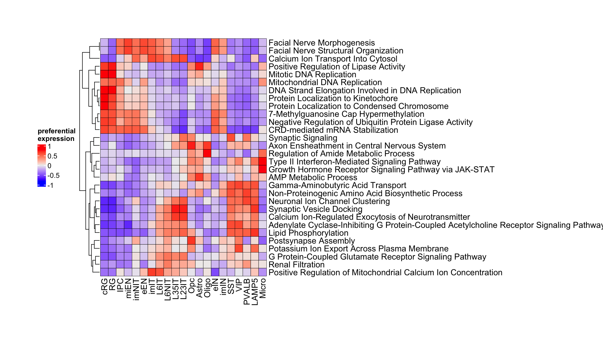

Figure 3.18: Top gene ontology biological processes in corticogenesis.

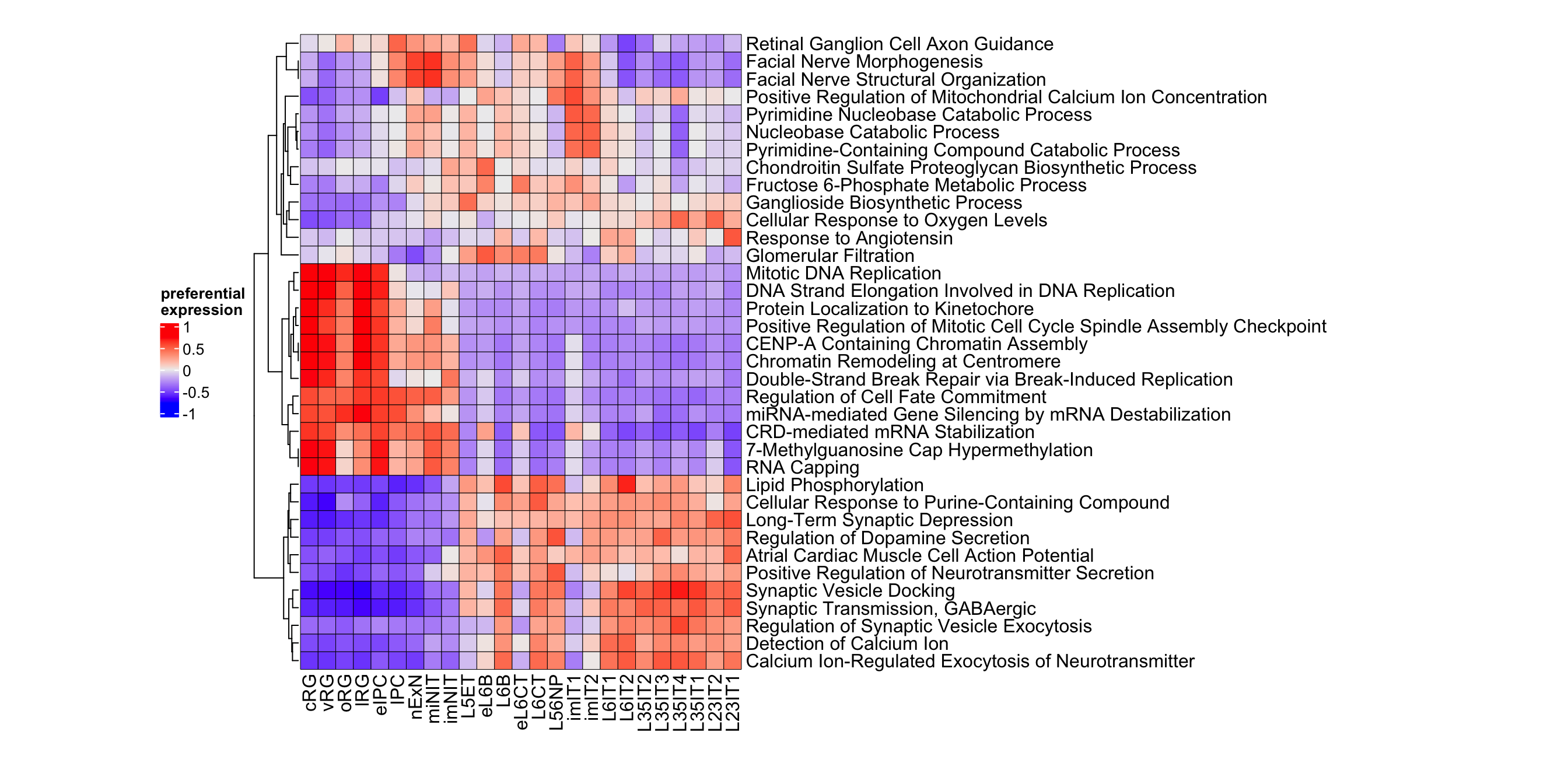
Figure 3.19: Top gene ontology biological processes in neurogenesis.

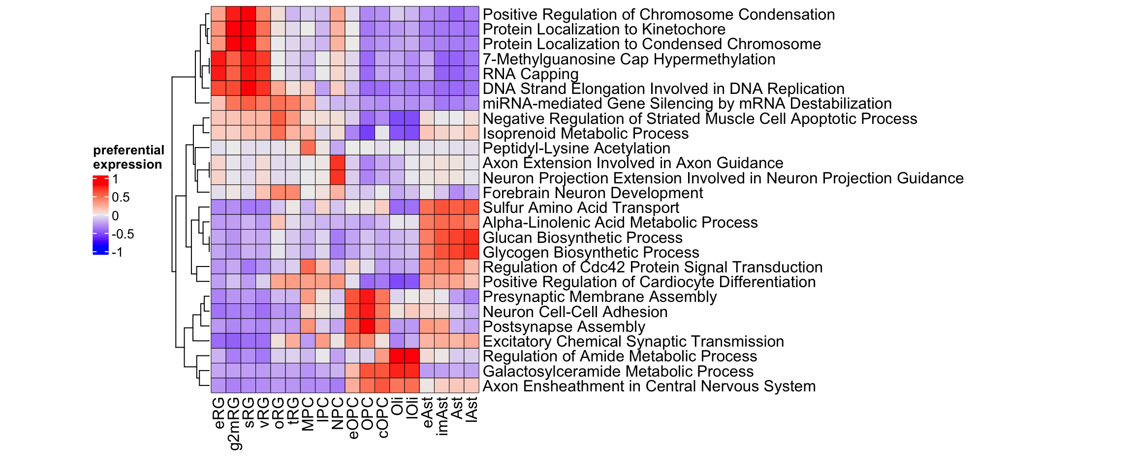
Figure 3.20: Top gene ontology biological processes in gliogenesis.

To focus on corticogenesis-relevant processes we have also manually curated a list of Gene Ontology Biological Processes for the corticogenesis and neurogenesis networks, available for download here (PreferentialExpression folder).

2 Network exploration

4 Mapping Bulk data